Determining the detailed temperature structure of the solar atmosphere from observations is a basic means of constructing and testing atmospheric models. One avenue to address this problem is based on measuring the center-to-limb variation of the intensity in various spectral regions. Observations in the radio domain are particularly suited for such a task since they don’t suffer from a set of complications (e.g., departures from the ionization and local thermodynamic equilibrium, elemental abundances) which may be relevant to the diagnostics in other wavelength domains. Another convenient aspect is that the quiet Sun radio emission is due to the free-free process (e.g., Shibasaki et al. 2011; Wedemeyer et al. 2016). We have recently performed such a study (Alissandrakis et al. 2017), using the Atacama Large Millimeter/submillimeter Array (ALMA).
Observations and Analysis
We analyzed ALMA observations at 100 and 239 GHz taken from the 16-20th of December 2015, a period of solar commissioning activities. Full disk (FD) images were constructed by scanning the solar disk with twenty 12-m antennas, using the compact configuration of ALMA. The full width at half maximum of the single dish beam is ~27” and 60” at 239 GHz and 100 GHz, respectively. The pipeline of solar observations with ALMA is described in White et al. (2017).
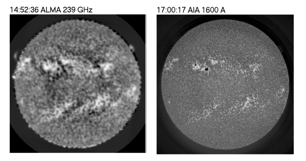 Figure 1. ALMA 239 GHz (left panel) and AIA 1600 Å (right panel) FD images, partly corrected for center-to-limb variation to enhance the visibility of disk features and prominences, taken during December 17, 2015 (from Alissandrakis et al. 2017).
The left panel of Figure 1 contains a sample ALMA FD image at 239 GHz. Several basic features of the chromosphere can be readily discerned in the image: plage regions, a big sunspot, prominences and finally the chromospheric network. As a matter of fact, the chromospheric network structure observed at 239 GHz bears a strong resemblance with chromospheric/transition-region AIA images at 1600 Å (right panel of Figure 1).
In order to derive the center-to-limb variation (CLV), the average brightness temperature, $T_{b}$, as a function of radial distance $r$ was computed, ignoring too dark or too bright pixels, corresponding to filament channels and plage regions; regions too close to the limb were also ignored.
The formal solution of the radiative transfer equation in the radio domain is:
\[T_{b}(\mu)=\int_{0}^{\infty}T_{e}(\tau)e^{-\tau/\mu}d\frac{\tau}{\mu}\]
where $T_{e}(\tau)$ is the electron temperature and $\tau$ is the optical depth, $\mu=cos\theta$, with $\theta={sin}^{-1}(r/R_{\odot})$. Given the ${f}^{-2}$ dependence of the absorption coefficients for both free-free and $\mathrm{H}^{-}$ emissions, we re-mapped accordingly our 100 and 239 GHz observations and also included the measurements of Bastian et al. (1993), at 353 GHz. The combination of the CLV curves for these three frequencies gave rise to a more extended range in $\mu$, and thus also in $\tau$.
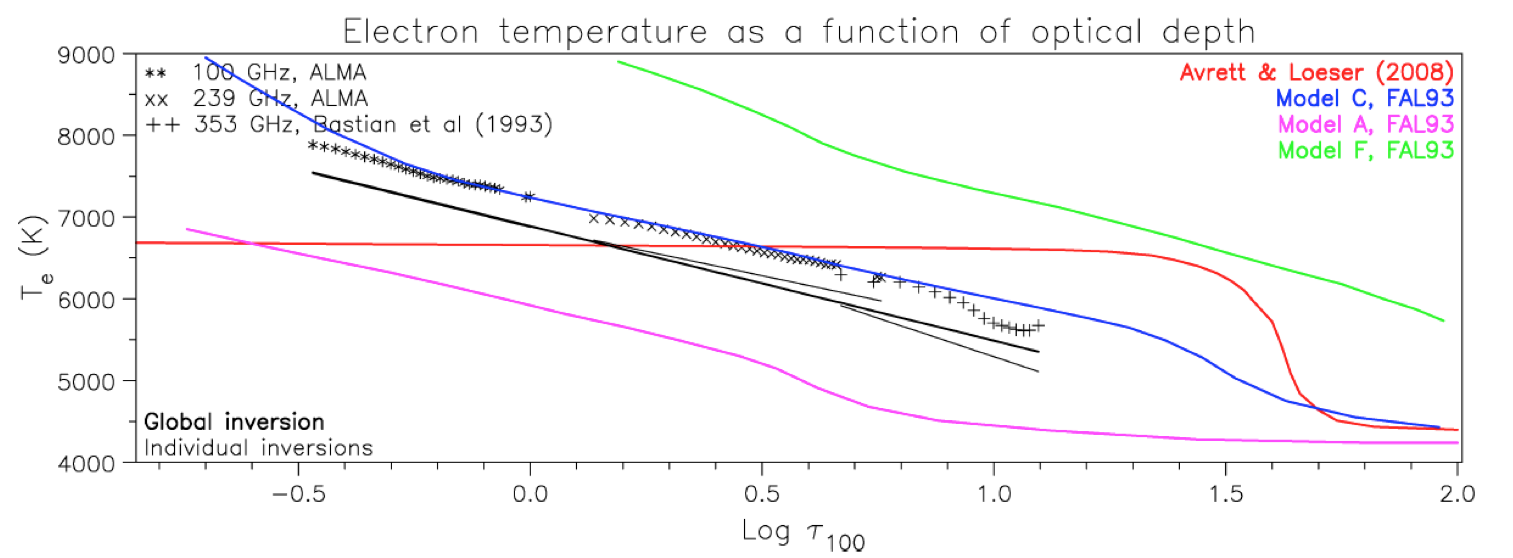 Figure 2. Electron temperature as a function of optical depth at 100 GHz. The thick black line is the result of the inversion of the ALMA CLV data, along with the data of Bastian et al. (1993). Thin black lines are inversions of individual wavelength bands. The symbols correspond to the familiar Eddington-Barbier solution of the radiative transfer equation. The full lines in color were computed from the models of Fontenla et al.(1993) and Avrett and Loeser (2008). From Alissandrakis et al. (2017).
In order to calculate $T_{e}(\tau)$ from the observed $T_{b}(\mu)$ one has to invert Equation 1. For this, we tried several functional forms of $T_{e}(\tau)$; best results were obtained with a linear dependence of $T_{e}$ on $\ln\tau$
The results of our inversions are displayed in Figure 2 (black lines), together with the predictions of the atmospheric models of Fontenla et al.(1993) and Avrett and Loeser (2008). Our inversion is in rather good agreement ($\sim5 \%$ lower) with model C of Fontenla et al. (1993); this model corresponds to the average quiet Sun, therefore combining the contributions of both network and cell interior. We note that the Eddington-Barbier solution (symbols) has a similar shape compared with our other inversion, albeit with an offset of 350 K; this is because the E-B approximation ignores the second-degree term in the Taylor expansion of $T_{e}(\tau)$.
Conclusions
Our study is the first effort to determine the thermal structure of the solar chromosphere using limb-brightening curves from ALMA. Our results suggest a satisfactory agreement with standard atmospheric models, and namely model C of Fontenla et al. (1993) and do not confirm previous results that the radio data are closer to the cell interior model A. Given the degrading effect of the antenna beam, it was not possible to deduce separate CLV curves for the network and cell interior in this study. This will be possible using interferometric observations of ALMA. This task, along with detailed comparisons with advanced radiative-MHD 3D models of the solar atmosphere (Wedemeyer et al. 2016) are important areas of future research.
References
Alissandrakis, C. E., Patsourakos, S., Nindos, A., Bastian, T.: 2017, A&A in press See https://doi.org/10.1051/0004-6361/201730953
Avrett, E. H., Loeser, R.: 2008, ApJS, 175, 229
Bastian, T. S., Ewell, M. W., Zirin, H.: 1993, ApJ, 415, 364
Fontenla, J. M., Avrett, E. H., Loeser, R.: 1993, ApJ, 406, 319
Shibasaki, J., Alissandrakis, C. E., Pohjolainen, S.: 2011, Sol. Phys., 273, 309
Wedemeyer, S., Bastian, T., Brajša R., et al : 2016, SSRv, 1, 200
White, S. M., Iwai, K., Phillips, N. M., et al.: 2017, Sol. Phys., 292, 8
*Full list of authors: Costas Alissandrakis, Spiros Patsourakos, Alexander Nindos, Tim Bastian