The solar flare phenomenon is a complex process in the solar atmosphere where non-potential magnetic energy is released and converted into other forms of energy, such as nonthermal energy of accelerated particles, thermal energy of heated flaring plasma, kinetic energy of eruptions, jets, up/down flows, and stochastic (turbulent) plasma motions. The processes lying behind initial division between energy components, distribution of these components among flaring loops and their evolution are not yet fully understood. A recent statistical study by Lysenko et al. (2018) described a class of early impulsive ‘cold’ flares, where the direct heating is weak and most of plasma heating is driven by accelerated electrons. Such flares offer the cleanest way to study the electron acceleration in flares and the thermal plasma response driven by the nonthermal electron population.
Here we quantify the energy partitioning and spatial distribution in a SOL2014-02-16T064620 solar flare of class C1.5, which has relatively weak thermal response similar to cold flares. This event is a rare case when a rather simple flare with a ‘single-spike’ impulsive phase was observed with IRIS so we can quantify the kinetic energy of turbulent and bulk plasma motions in the flare footpoints.
Analysis of Observations
In the study we analyze SDO/AIA and RHESSI data to take into account both moderately heated and hot components of the flaring plasma in the coronal part of the flare. Applying the regularized inversion code to the SDO/AIA data (Hannah & Kontar 2012, 2013) and the methodology described in Motorina et al. (2020) we calculate the spatial distribution of temperature, emission measure, and thermal energy density (Figure 1, a). The main contribution to the thermal energy comes from the flare area (box 2 in Figure 1, a, upper left panel) which can be divided into two regions (marked with green/magenta lines) corresponding to two different flaring loops. The bulk of the thermal energy contained in the flare region is equally divided between these two loops (Figure 1, b). Evolution of this energy (from box 2) is shown in Figure 1(c) in black with its peak value at ~7×1028 [erg].
Given that RHESSI missed the impulsive phase due to being in the orbital night, we use the X-ray data from RHESSI only in the decay phase. To calculate the thermal energy detected by RHESSI, we use the emission measure and temperature obtained from the RHESSI fit and volume of the corresponding Loop II from a 3D flare model. The evolution of this energy is shown in Figure 1(c) in green with the peak value of ~5×1028 [erg].
Hard X-ray observations of the impulsive phase are only available in the Konus-Wind wide G1 channel covering 21–80 keV range. These observations in conjunction with the NoRP, RSTN, and BBMS data in microwave range and a built 3D model of the flare are employed to estimate the nonthermal energy deposition in the flare (Figure 1, c, blue line). The nonthermal energy deposition derived from the RHESSI fit (Figure 1, c, dark blue dashed line) during the decay phase does not contradict any available data.
The IRIS data show activity (impulsive enhancements in the flare area) temporally coinciding with the impulsive emission from Konus-Wind and microwaves. We analyze the spectral lines Si IV, O IV, and Fe XXI which form at different transition region to coronal temperatures. We fit a Gaussian function to each pixel for each spectral line to determine their Doppler velocities and Doppler widths and thus to quantify the kinetic energy of the plasma flows and turbulent motions. Because of weak signatures of Fe XXI, we cannot use this spectral line to estimate a coronal portion of the kinetic energy. The considered temperature range 104.8-105.1 K belongs to the flare footpoints. Thus, these data quantify only a fraction of the total kinetic energy in the flare. We determine which IRIS pixels lie inside the 50% RHESSI 6-9 keV contour and calculate this energy 3 × 1024 [erg]. Then we found the total turbulent kinetic energy for the same volume as less than 7 ×1025 [erg].
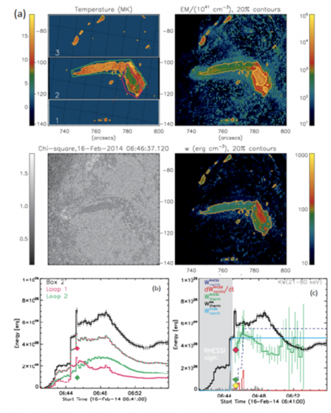
Figure 1 – (a) Spatial distributions of plasma parameters derived from SDO/AIA: temperature (top left panel), emission measure (top right panel), chi-square (bottom left panel), thermal energy density (bottom right panel). (b) Components of the thermal energy inside box 2 defined in Figure 1(a): green/magenta lines correspond to green/magenta ROIs. The red and green symbols indicate the model values of thermal energies Loops I and II, respectively. (c) Evolution of the energy components in the February 16, 2014 flare.
3D Modeling
Based on the NLFFF extrapolation code (Fleishman et al. 2017) initiated with an SDO/HMI vector magnetogram taken at 06:34:12 UT and GX Simulator (Nita et al. 2015) we built a 3D flare model (Figure 2). The GX Simulator functionality permits computation (and visualisation) of selected magnetic field lines such as to match available flare images. With the use of the AIA and RHESSI images we identified three loops and filled them with thermal plasma. The red, green, and yellow symbols in Figure 1 (c) indicate the model values of thermal energies in Loops I, II, and III respectively.
Based on the only available microwave spectral data at 06:44:41UT we found that energetically dominant fraction of the nonthermal electrons must be located in Loop II. The built model is consistent with all available observational constraints and, thus, validated by the data.
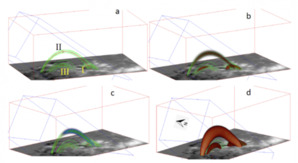
Figure 2 – The 3D model with three flux tubes labeled with their numbers (I–III). (a) Magnetic flux tubes. (b) Distribution of thermal number density in the flux tubes. (c) Distribution of nonthermal number density in the flux tubes (in Loop II only). (d) Distribution of the temperature in the flux tubes.
Conclusions
In this study, we have analyzed the SOL2014-02-16T064600 flare which has three distinct consecutive heating episodes, where the second one appeared as a response on the nonthermal impulsive peak. From the timing of the event, we can conclude that only a portion of the flaring plasma heating was driven by nonthermal electron losses, while the remaining portion was driven by another agent.
We found that the flare occurred in a multi-loop system that included at least three distinct flux tubes. The nonthermal electron population was only detectable in the largest and hottest Loop II, while two other loops remained thermal. The distribution of the energy components over the three flaring loops involved in the event was highly uneven. The accounted forms of the kinetic energy in the flare footpoints constituted only a minor fraction compared with the thermal and nonthermal energies.
Nonthermal energy input was sufficient for the postimpulsive heating in the flaring loop with nonthermal electrons, but insufficient for the overall thermal response in the flare.
Based on the recently published paper: Gregory D. Fleishman, Lucia Kleint, Galina G. Motorina, Gelu M. Nita, and Eduard P. Kontar, Energy budget of plasma motions, heating, and electron acceleration in a three-loop solar flare, The Astrophysical Journal, 913, 97 (2021) (https://doi.org/10.3847/1538-4357/abf495)
References
Hannah I.G. & Kontar E.P. 2012, A&A, 539, A146 https://doi.org/10.1051/0004-6361/201117576
Hannah I.G. & Kontar E.P. 2013, A&A, 553, A10 https://doi.org/10.1051/0004-6361/201219727
Lysenko A.L. et al. 2018, ApJ, 856, 111 https://doi.org/10.3847/1538-4357/aab271
Motorina G.G. et al, 2020, ApJ, 890, 75 https://doi.org/10.3847/1538-4357/ab67d1
Fleishman G.D. et al. 2017, ApJ, 839, 30 https://doi.org/10.3847/1538-4357/aa6840
Nita, G. M. et al. 2015, ApJ, 799, 236 https://doi.org/10.1088/0004-637X/799/2/236
*Full list of authors: Gregory D. Fleishman, Lucia Kleint, Galina G. Motorina, Gelu M. Nita, and Eduard P. Kontar