Despite many years of study, the dominant driver and energy source of coronal mass ejections (CMEs) is still under investigation. Observational studies have indicated that magnetic energy represents the largest part of the total energy budget of the eruption (Emslie et al., 2012, Carley et al., 2012). However, despite having such a dominant influence on CME dynamics, little is known about CME magnetic field. This is due to the scarcity of measurements of this CME property. Therefore, any new measure of this quantity represents a rare and important diagnostic that is essential for gaining a complete picture of CME evolution. In this study we report on a rare combination of radio and X-ray observations from non-thermal electrons associated with the development of a CME in the low corona. This combination of observations allows us to estimate the magnetic field associated with the CME core.
Gyrosynchrotron emission sources at the onset of a CME
The SOL2014-09-01 event was associated with a flare occurring 36$^{\circ}$ beyond the east solar limb and a fast coronal mass ejection (~2000 km$\,$s$^{-1}$). Beginning at 11:00 UT, the Nançay Radioheliograph (NRH) observed an unusually large source of radio radiation from 150-445 MHz at the same location as the eruption, see Figure 1a. All frequencies are located at the same position on the plane-of-sky (POS), which is not expected of plasma emission. Figure 1b also shows the similarity of the expansion of the CME internal loops (at the core) and the expansion of the radio sources, indicating the radio emission likely belongs to the CME core.
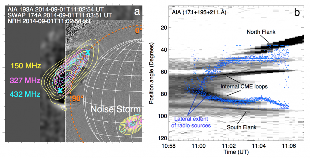 Figure 1. (a) Extreme ultraviolet (EUV) difference images of an eruption off the east limb, observed using the Atmospheric Imaging Assembly (AIA) and the Sun Watcher using Active Pixel System detector and Image Processing (SWAP). Superimposed on the image are the contours of a large radio source observed in NRH from 150 to 445 MHz (just three frequencies are shown here). (b) Position angle expansion over time of the CME, with internal loops and CME flanks indicated. The blue points demarcate the position angle extent of the 432 MHz radio source (shown by the two ‘x’ symbols in panel a). The radio source and CME internal loops have closely correlated expansion.
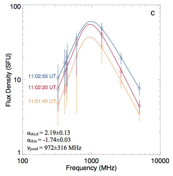 Figure 2. Flux density measurements of the source from NRH (<445 MHz) and RSTN (>610 MHz) show a gyrosynchrotron spectrum, three different times are shown. Frequencies below 300 MHz observed by NRH were mainly plasma emission and not shown here.
Using flux density measurements of the sources imaged using NRH along with observations from the Radio Solar Telescope Network (RSTN), a flux density spectrum was constructed, see Figure 2. These data were fit with a parametric expression for a gyrosynchrotron flux density spectrum (Stahli et al., 1989), allowing for an estimate of frequency of peak emission ($\nu_{peak}=1\,$GHz) and the spectral indices $\alpha_{thick}=2.19\pm0.13$ and $\alpha_{thin}=-1.74\pm0.03$, which are indicative of a non-thermal gyrosynchrotron spectrum (Nita et al., 2004). Now, from Dulk & Marsh (1982) the magnetic field strength at the radio source may be estimated from
\( \nu_{peak} \approx 2.72 \times 10^{3} 10^{0.27\delta} (\sin\theta)^{0.41+0.03\delta}(NL)^{0.32-0.03\delta} \times B^{0.68+0.03\delta} ~~~~~ (1) \)
where $\theta$ is the angle between the line-of-sight (LOS) and the magnetic field direction, $N$ is the non-thermal electron density, $L$ is the LOS length of the radiating source and $B$ is the magnetic field strength at the radio source location; $\delta$ is the spectral index of the electrons in the power-law distribution (e.g., where the distribution in energy follows $E^{-\delta}$) and is related to the optically thin spectral index of the flux density spectrum by \(\delta = |-1.1(\alpha_{thin}-1.2)|\), resulting in \(\delta=3.2\pm0.3\). We choose $\theta$$\sim$45$^{\circ}$ (from considerations of the observed low polarisation of radiation, see Carley et al., 2017) and $L$$\sim$0.45 R$_{\odot}$ (from the radio source POS size in NRH images). The remaining unknown is $N$, the number density of non-thermal electrons in the radio source. We have no independent measure of this using radio observations. However, we may calculate $N$ using X-ray observations at the time of the event. Use of $N$ from X-ray observations in a calculation of radio gyro-emission is initially motivated by the close spatial relationship that radio and X-ray sources have in images, see Figure 3a. Furthermore such a combination of X-ray and radio analysis is only valid if we can show that the radio and X-ray emissions come from the same distribution of energetic electrons.
X-ray and radio emitting CME electrons
Figure 3a shows the X-ray observations at the time of the event, with an image from GOES Soft X-ray Imager (SXI). The FERMI Gamma-ray Burst Monitor (GBM) also observed X-ray flux from 4-50 keV, enabling a photon energy spectrum to be calculated (see Carley et al., 2017). Given that the event was behind the limb, we fit the photon spectrum with a model of an optically thin thermal component combined with a thin-target source. Interestingly, the electron spectral index derived using X-ray observations ($\delta=2.9\pm0.5$) is similar to that derived from radio ($\delta=3.2\pm0.3$). The similarity of these indices and the close spatial relationship of the radio and X-ray sources in images indicates that the X-ray and radio emitting electrons may come from a similar population. This provides us with an opportunity of estimating the non-thermal number density $N$ from X-rays and using this in Eqn 1 above to find the magnetic field strength $B$.
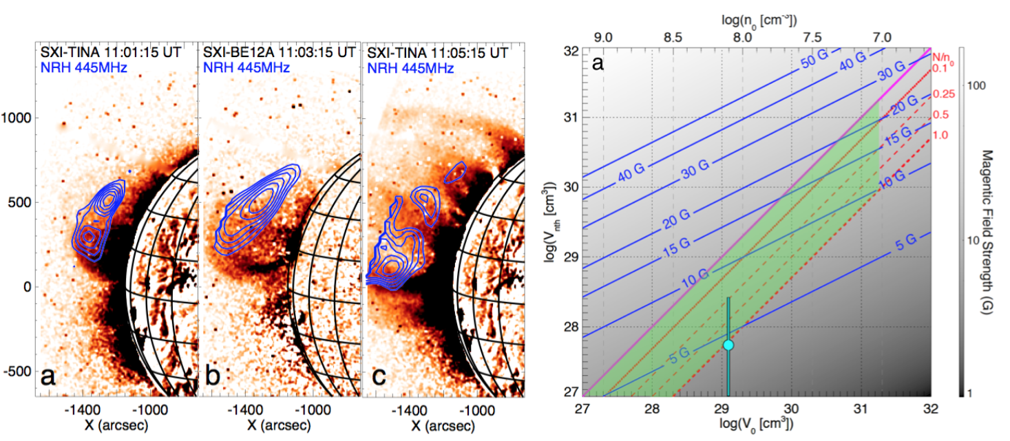 Figure 3: (a) GOES SXI difference images of the erupting source with NRH 445 MHz contours, showing a close spatial relationship. (b) Solution space of magnetic field strengths (indicated by contours), as a function of X-ray source volumes $V_0$ and $V_{nth}$. Specific ratios of thermal to non-thermal electron densities $N/n_0$ are indicated in red. The green shaded region is the space of physically meaningful values for $B$, given particular physical constraints.
Estimating magnetic field strength using radio and X-rays
From the thin-target model fit to the GBM photon spectrum, we are able to estimate a value for $N$ via the equation
\(N=\frac{[n_{0}V_0\overline{F}]}{n_{0}V_{nth}}\frac{\delta-1}{\delta-0.5}E_{min}^{-1/2}\sqrt{ \frac{m}{ 2 } } \bigg( \frac{E_0}{E_{min}} \bigg)^{\delta-1} ~~~~~ (2) \)
where \( n_{0}=\sqrt{\frac{\xi}{V_0}} \), $\xi$ is the emission measure, $V_0$ and $V_{nth}$ are thermal and non-thermal X-ray source volumes, respectively, $N$ is non-thermal electron number density, $[n_{0}V_0\overline{F}]$ is the integrated electron flux, $\delta$ is electron spectral index, $E_{0}$ is the energy above which there is a power-law distribution, $E_{min}$ is the energy above which the electron density is to be calculated, and $m$ is electron rest mass. $[n_{0}V_0\overline{F}]$, $\xi$, $\delta$, and $E_{0}$ are known from the above thin-target model fit to the GBM photon spectrum.
The remaining unknowns are $V_0$ and $V_{nth}$. Based on observations of the thermal source sizes in the Xray images we choose a range of $V_{0}$=$V_{nth}$=$10^{27}-10^{32}\,$cm$^{3}$. Now, due to the magnetic field strength $B$ dependence on $N$ (Eqn 1), which in turn depends on both $V_0$ and $V_{nth}$ (from Eqn 2), we may construct a solution space of $B(V_0, V_{nth})$, and use physical constraints to calculate reasonable values for $B$, see Figure 3b. For example, we apply physical constraints on the X-ray volume sizes and also ratios of non-thermal to thermal electron density, such that $V_{nth}<V_0$ and $N/n_0 <1.0$. These constraints define the shaded green region in Figure 3b, giving a magnetic field strength in the range if $B=4–25$ G. In order to verify these findings, we separately employ a full gyrosynchrotron numerical model developed by Simões & Costa (2006). The gyrosynchrotron model fit to radio spectrum indicates more precisely a magnetic field strength of 4.4$\pm$2.7 G (indicated by the blue point in Figure 3b), which falls within the range of the field strength estimated from Eqn 1. The gyrosynchrotron modelled B-field is indicated by the blue point in Figure 3b.
Finally, we use the numerical model to estimate the energy range of the electrons that produce the gyrosynchrotron radiation. It indicates that the electrons have a spectral index of $\delta=3.2$ (similar to that calculated above), with an energy in the range of 1-6 MeV. This suggests that the radio and X-ray emission in this event come from a similar population of electrons of spectral index $\delta\sim3$, with the X-rays originating in the lower energy part of the distribution (on the order of 10 keV), and the radio originating in the higher energy part of the distribution (on the order of 1 MeV).
Conclusions
This study detailed the observation of a large behind the limb flare and CME associated with an extended radio source observed by NRH, being identified as gyrosynchrotron emission when combined with RSTN observations. The event was also associated with HXR observations from FERMI GBM and X-ray imaging observations of the eruption using GOES SXI. This unique set of X-ray and radio observations allowed us to diagnose both the CME magnetic field strength and a variety of energetic electron properties including number density, spectral index and energy ranges which contribute to the radio and X-ray emission. A magnetic field strength of 4.4 G at a CME core height of 1.3 R$_{\odot}$ is similar to the values of CME magnetic field found previously (e.g., Bain et al. 2014). Finally, while all studies to date give some suggestion as to the location of the magnetic field strength measurement within the CME e.g., front, core or flank, no information exists to date on the spatial distribution and relative strengths of the magnetic fields in different parts of a CME. Future observations or instrumentation should aspire to such measurements. For the moment, magnetic field measurements in CMEs remain the most important yet elusive diagnostic in CME physics.
Additional info
Based on recent publication, Carley et al., 2017, A&A, 608, A137. https://doi.org/10.1051/0004-6361/201731368
References:
Carley, E. P., et al., The Astrophysical Journal, Volume 752, Issue 1, article id. 36, 8 pp. (2012).
Stahli, M., et al., Solar Physics (ISSN 0038-0938), vol. 120, no. 2, 1989, p. 351-368. (1989).
Nita, G. M., et al., The Astrophysical Journal, Volume 605, Issue 1, pp. 528-545. (2004).
Bain, H. M. et al., The Astrophysical Journal, Volume 782, Issue 1, article id. 43, 12 pp. (2014).
*Full list of authors: Eoin P. Carley, Nicole Vilmer, Paulo J. A. Simões, and Brían Ó Fearraigh