Solar spicules were discovered by the Jesuit priest Angelo Secchi in 1877. They are small plasma jets of a few hundred kilometers in diameter that are launched to heights >10 Mm with speeds ranging from a few 10s of km/s to >100 km/s. Individually they have lifetimes of a few minutes. They occur in the chromospheric network over the entirety of the Sun. Early estimates (Beckers 1972) suggested that spicules carry an upward mass flux 100 times that required to replenish losses from the corona due to the solar wind. With the advent of modern, high-resolution observations from space using Hinode SOT (optical), IRIS (UV), and SDO AIA (EUV), coupled with advanced modeling, there has been a resurgence of interest in spicules and their possible role in the mass and energy budget of the solar atmosphere.

Observations at millimeter wavelengths (mm-$\lambda$) are highly complementary to those in the O/UV/EUV bands. This is because the spicule emission is free-free from thermal electrons in LTE, the source function at mm-$\lambda$ is Planckian and the Rayleigh-Jeans approximation is valid. In contrast, O/UV lines form in non-LTE. Observations of the Sun in general and spicules in particular at mm-$\lambda$ were hampered by a lack of angular and temporal resolution. With the availability of ALMA, that has now changed. ALMA can image spicules with arcsec resolution and can resolve their kinematics with high cadence imaging.

Here, we briefly summarized ALMA observations of solar spicules in a polar coronal hole. Details may be found in the recently published paper by Bastian et al. (2025) or the arXiv reprint.

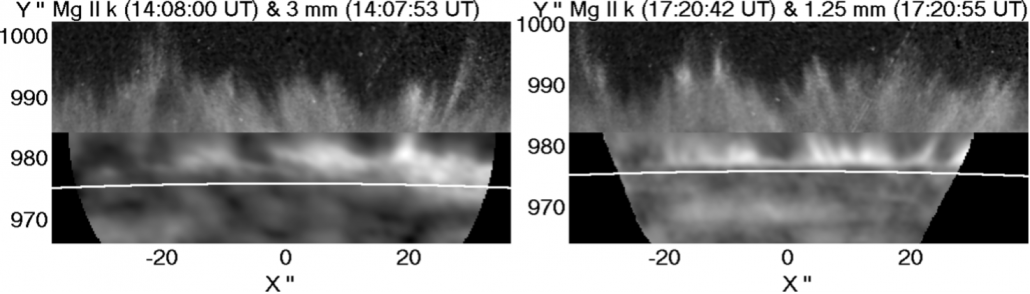
Figure 1. A comparison between ALMA and IRIS observations. Left: Spicules seen in 3 mm (lower part) and by the IRIS slit-jaw imager in the 2796Å band (upper part). Right: The same, but the lower part of the composite shows the 1.25 mm emission. The white arc indicates the photospheric limb.

ALMA Observations

The ALMA observations of solar spicules in the north polar coronal hole were obtained on 2018 December 25 in the 3 mm band over a field of view of approximately 60” with a cadence of 2 s, and in the 1.25 mm band over a similar field of view with a cadence of nearly 2 min. The reason for the slow cadence of the 1.25 mm images is that mosaicking techniques were used to combine 14 discrete pointings at this wavelength to produce a field of view comparable to that of the 3 mm band. As ALMA cannot observe in two frequency bands simultaneously, the 3 mm observations preceded the ones at 1.25 mm by about 3 hours.

We measured the variation of brightness temperature with height for an ensemble of spicules in both mm-$\lambda$ bands. If the temperature of the spicular plasma is known, the optical depth can be inferred as a function of height, from which the column density can be inferred and, hence, the electron number density $n_e$. We assumed two schematic models for the variation of spicule temperature with height: a) that it was isothermal; b) that the temperature increased linearly to transition region values. It is important to note that densities inferred from mm-$\lambda$ emission are remarkably insensitive to the plasma temperature, with $n_e \propto T_e^{1/4}$. Whatever its temperature, the ALMA observations capture the density of spicular material.

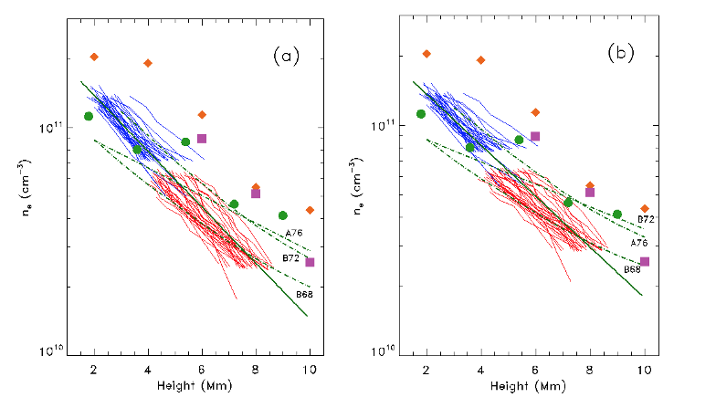
Figure 2: Spicule densities inferred from the mm-$\lambda$ observations. Densities based on 1.25 mm measurements are shown in blue and those based on 3 mm measurements are shown in red. a) Spicules are assumed to be isothermal with a temperature of $1.5\times 10^4$ K. b) Spicules are assumed to have a temperature of $1.5\times 10^4$ K at a height of 2 Mm, increasing linearly to $10^5$ K at a height of 15 Mm. In both panels, the solid green line represents the fit to the aggregated 1.25 and 3 mm data. The data points are from Alissandrakis et al. (2018) (filled green circles), Beckers (1972) (purple squares), and from Krall et al. (1976) (orange diamonds). The dash-dot lines labeled “B68″, “B72″, and “A76″ are the densities resulting from spicular filling factors based on the model of Beckers (1968, 1972), and Athay (1976), respectively.

We find that spicular densities derived from the dual-band mm-$\lambda$ observations compare well with those inferred from historical O and UV observations. When the line-of-sight filling factor is taken into account, the variation of density with height is somewhat flatter (dashed lines in Figure 2). We also find that the upward mass flux due to spicules falls rapidly with height, calling into question whether they play a significant role in the mass budget of the solar corona and solar wind. However, we cannot exclude the idea that electrical currents or wave modes carried by spicules may play a role in transporting energy into the solar corona.

Conclusions

ALMA observations at mm-$\lambda$ provide new insights into a variety of solar phenomena, including solar spicules. Our results do not provide support for the idea that spicules provide significant mass to the corona. Nevertheless, additional work is very much needed: multi-band observations of spicules in a variety of environments (coronal holes, quiet Sun) as well as detailed quantitative comparisons with observations made at O/UV/EUV wavelengths.

Based on the recent paper by T. S. Bastian, C. Alissandrakis, A. Nindos, M. Shimojo, and S. M. White, ALMA Observations of Solar Spicules in a Polar Coronal Hole, ApJ 980 60 (2025). DOI:10.3847/1538-4357/ada445

References

Alissandrakis, C., et al. 2018, Solar Phys. 293, 20 doi: 10.1007/s11207-018-1242-4

Anthay, R. G., 1976 “The solar chromosphere and corona: Quiet sun”, Vol. 53, doi: 10.1007/978-94-010-1715-2

Bastian, T. S., Alissandrakis, C., Nindos, A., Shimojo, M., and White, S. M. 2025, ApJ 980, 60, doi: 10.3847/1538-4357/ada445.

Beckers, J. 1968 SoPh, 3, 367, doi: 10.1007/BF00171614

Beckers, J. 1972, ARA&A, 10, 73, doi: 10.1146/annurev.aa.10.090172.000445

Krall, K. R., Bessey, R. J., & Beckers, J. M. 1976, SoPh, 46, 93, doi: 10.1007/BF00157556