Traveling ionospheric disturbances (TIDs) are one particular type of the Earth’s ionosphere irregularities (Hunsucker, 1982). They represent wave-like electron density structures propagating in the ionosphere. The motion of TIDs modulates the electron density distribution in space. It leads to a modification of plasma parameters, namely the refractive index, and affects the propagation of radio waves. In particular cases, the variations of plasma parameters strongly affect the lower-frequency electromagnetic waves that can result in focusing or amplification of the incident radiation (Meyer-Vernet et al. 1981). The focusing effect manifests itself in the form of peculiar spectral disturbances in intensity with specific morphology, so-called Spectral Caustics (SCs), occasionally appearing in dynamic spectra of different solar radio instruments operating in the meter-decameter wavelength range (CESRA nugget by Koval et al.).
In this study, for the first time we present simulation results of the focusing effect of the medium scale traveling ionospheric disturbances (MSTIDs), on solar radio emission by applying a ray-tracing method to the Earth’s ionosphere with MSTIDs. To simulate the day-time MSTIDs, we have considered the typical parameters of a TID having a horizontal wavelength λ of 300 km, temporal period T of 40 min (see Figure 1). Then, radio rays trajectories in the modeled ionosphere have been calculated by using an algorithm based on the piecewise linear approximation of the smooth trajectory of a beam, in which the ionosphere is divided into layers, and the direction of the refracted beam is found with the Snell’s law.
Simulation Results
In Figure 1, two representative examples of refraction of radio waves (radio rays) at frequencies 105 MHz (a) and 75 MHz (b) in the modeled ionosphere are shown. The rays come out from points distributed between 1600 and 2000 km with a 4-km step along horizontal distance and placed at 450 km in altitude. The elevation angle θ is equal to 8⁰. Each panel presents a picture of radio rays at the same instant with the only difference in radio wave frequency. At a receiving point located at the ground level the number of incoming radio rays is counted. In the figure, the selected range of distances (cell) – 700-704 km – is marked by purple asterisk, while the purple histogram bars indicate the number of rays getting into this distance range. An increase of the number of radio beams in the cell up to 16 for 105 MHz and up to 3 for 75 MHz is registered.
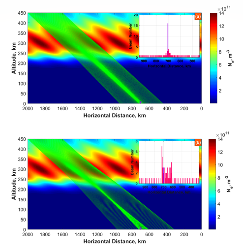 Figure 1. Examples of the simulations of the propagation of radio rays (green lines) at 105 MHz (a) and 75 MHz (b) through the perturbed ionosphere. The rays are uniformly distributed in the range of distances from 1600 to 2000 km with 4 km spacing. The starting point in altitude is 450 km. The elevation angle is equal to 8⁰. The histograms in both panels demonstrate the number of beams falling into the 4-km distance at the ground level. The histogram bin width is 4 km.
Figure 2 shows the main result of our calculations. Here the beam density has been increased by reducing the beam spacing to 1 km. Therefore, the number of incoming beams in 1-km distance at the ground surface was counted, while the propagation of TIDs with the spatial period of 300 km is simulated by moving the structures every 1/300 of the temporal period T, i.e. 40/300 min = 2/15 min. At the same time by changing the frequency of radio rays with a 1-MHz incremental step, we recorded the beam intensity in the time-frequency domain. In such a way we simulated the solar dynamic spectra for elevation angles θ equal to 2°, 8°, 14°, and 20°. Each dynamic spectrum includes distinctive spectral perturbation in intensity that can be recognized as a SC.
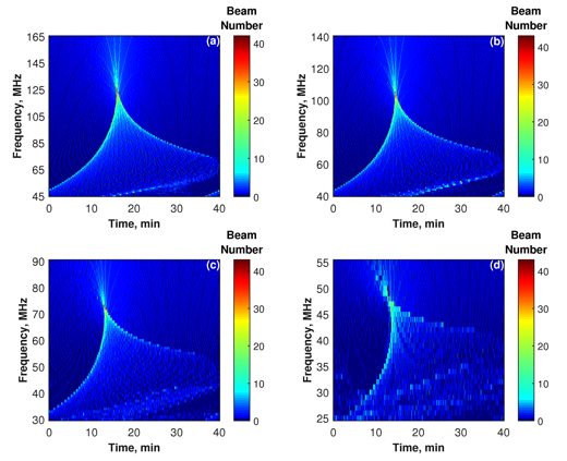 Figure 2. The beam-intensity in the time-frequency plane (i.e. dynamic spectrum) obtained by counting numbers of radio rays received in the fixed 1-km distance at the Earth’s surface (at the presumed observational site). The simulation is performed with 1 MHz resolution in frequency and 2/15 min resolution in time. The dynamic spectra were produced under different solar elevation angles: (a) 2⁰, (b) 8⁰, (c) 14⁰, (d) 20⁰. The color scale indicates the number of beams recorded at the presumed site of observation.
With the simulation, we are able to identify four types of SCs among the five ones declared by our earlier study, including the inverted V-like, V-like, X-like, and fiber-like types (Koval et al. 2017). This proves, firstly, the reliability of the introduced classification of the SCs; secondly, the correct numerical treatment of the issue; thirdly, further studies are required for explanation of the last type of SCs, i.e., the fringe-like type.
From Figure 2, it is seen that a typical SC structure consists of front and back envelopes and a body between them. The envelopes have higher brightness than the interior and approach each other at a certain convergent point that is characterized by the peak brightness of the whole structure. The frequency of the convergent point is the focusing frequency. It implies that with current parameters of the ionosphere and solar radiation a ground observer is in the focus of a plasma lens formed by TIDs. In Figure 2(a-d) it happens at frequencies of 125 MHz, 105 MHz, 73 MHz, 48 MHz, respectively. The dependency of the focusing frequency on solar elevation angle is presented in Figure 3.
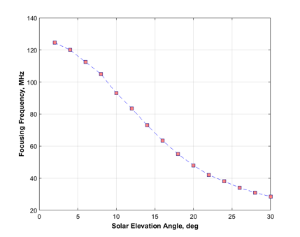 Figure 3. Dependency of the focusing frequency on the elevation angle of the Sun. The values of the focusing frequency (orange squares) are determined every 2⁰.
Figure 3 shows that the focusing frequency rapidly falls with the growth of the elevation angle. The low values of the elevation angle correspond to typical positions of the Sun in winter and partially in spring and autumn months at middle latitudes of Europe. Based on the simulation result in Figure 2(d) for θ = 20⁰, a SC at larger θ would be partially or completely damaged, or not be generated at all. Thus, we infer that the SCs may be observed only in certain periods, mainly in late fall, winter, and early spring.
Conclusions
The simulation of the propagation of a plane electromagnetic wave through the terrestrial ionosphere with TIDs has been performed by application of geometrical optics. The main advantage of this approach is getting the full picture of radio rays trajectories. This visually shows a formation of caustics in space under different conditions of radiation source or/and ionosphere. It has been exhibited for the first time. Also we revealed that the SCs may be recorded in spectrograms for certain elevation angles of the Sun. At relatively low solar elevation angles (<25⁰), the SCs can be generated. This range of elevation angles corresponds to late fall, winter, and early spring. This provides a nice explanation of the seasonal dependence in SC occurrence which has been established in our previous paper (Koval et al. 2017). We believe this modeling work, which has also an elucidative character, is highly necessary to gain a better understanding of the focusing effect that is still little-known to communities of solar and ionospheric scientists.
Based on a recently published article: Koval, A., Chen, Y., Stanislavsky, A., Kashcheyev, A., & Zhang, Q.-H. (2018). Simulation of focusing effect of traveling ionospheric disturbances on meter-decameter solar dynamic spectra, J. Geophys. Res. Space Phys. https://doi.org/10.1029/2018JA025584
References
Hunsucker, R.D.,Rev. Geophys. Space Phys., 20, p. 293, 1982
Koval, A., Chen, Y., Stanislavsky, & Zhang, Q.-H., J. Geophys. Res. Space Phys., 122, p. 9092, 2017
Meyer-Vernet, N., Daigne, G., and Lecacheux, A., Astronomy & Astrophysics, 96, p. 296, 1981
*Full list of authors: A. Koval, Y. Chen, A. Stanislavsky, A. Kashcheyev, and Q.-H. Zhang