CMEs can be the sources of space-weather disturbances. Shock waves expanding ahead of fast CMEs and associated flares are the probable sources of energetic protons. Two categories of CMEs have traditionally been identified depending on the presence of conspicuous chromospheric emissions during their development. Flare-associated CMEs erupt from active regions, carry stronger magnetic fields, can reach higher speeds and cause stronger space-weather disturbances. Non-flare-associated CMEs develop in eruptions of large “quiescent” filaments away from active regions, are mostly slower, and have considerable space-weather impact rarely. Exceptional events deserve attention.
The eruption of a “quiescent” filament on 29 September 2013 led to a fast CME (1180 km s$^{-1}$: CDAW CME catalog), caused a big near-Earth proton enhancement, Forbush decrease, and geomagnetic storm. We analyze why this non-flare-associated CME was so fast and how the shock wave was excited.
Kinematics and Reconnection Flux
The filament and CME components accelerated nearly simultaneously with a peak of the reconnection rate measured by Cliver et al. (2019) (Figure 1) that confirms responsibility of reconnection for the eruption. By comparing plane-of-the-sky images of the erupting filament with a radial component of the extrapolated magnetic field, we estimated the deprojected kinematics. The established deprojected speeds were 930 km s$^{-1}$ for the prominence top and 1305 km s$^{-1}$ for the frontal structure.
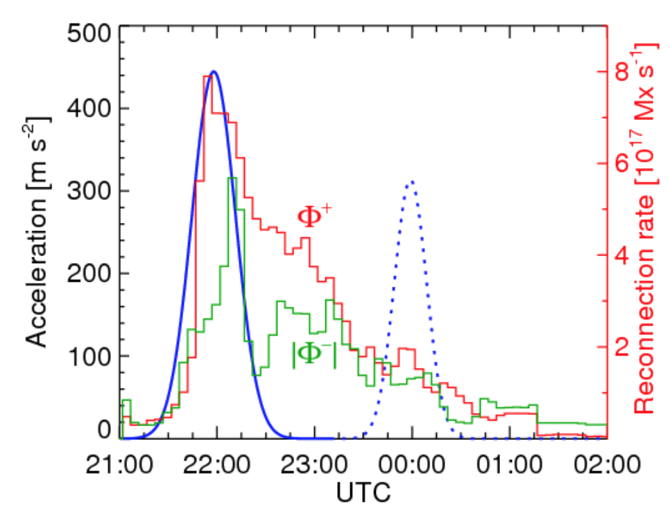 Figure 1 – Acceleration of the prominence/CME core (blue; solid: eruption, dotted: reacceleration at $8 R_{\odot}$ ) and reconnection rate (adapted from Cliver et al. (2019)).
Cliver et al. (2019) measured the total unsigned magnetic flux involved in this eruption of $\Phi_{\mathrm{tu}} = 6.4 \times 10^{21}$ Mx. The method by Chertok et al. (2017) gives a close estimate of $\Phi_{\mathrm{tu}} = 5.5 \times 10^{21}$ Mx. With a nominal brightness threshold of 5%, significant parts of the arcade are missed in this event. We reduced the threshold to 1% and considered both the arcade and ribbons at different times (Figure 2).
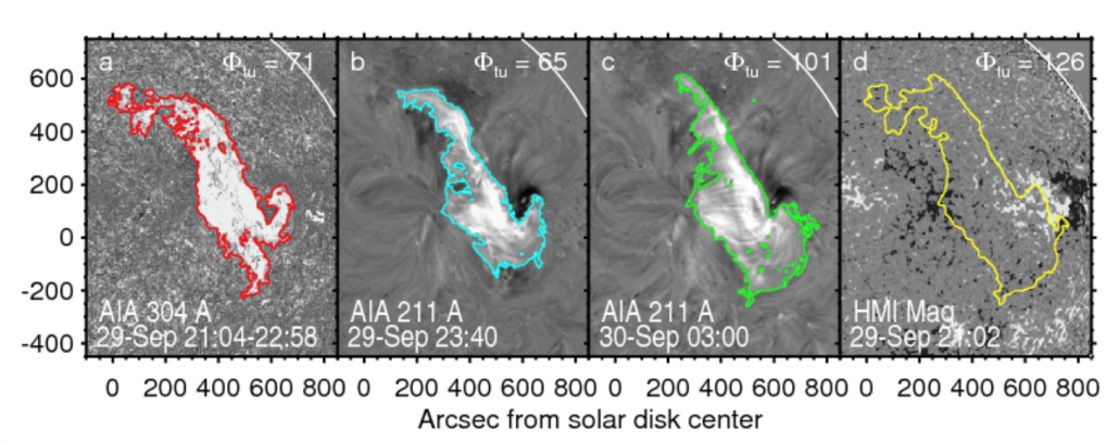
Figure 2 – (a-c) Total unsigned magnetic flux measured within the arcade (contours) identified from SDO/AIA images. (d) Combined areas in panels a-c (yellow contour) overlaid on the SDO/HMI magnetogram.
The magnetic flux estimated using the image in Figure 2b coincides with the estimate by Cliver et al. (2019) that confirms the equivalence of the two methods and justifies the decreased brightness threshold. The total magnetic flux within the yellow contour in Figure 2d that combines the areas in Figures 2a-2c is $\Phi_{\mathrm{tu}} = 12.6 \times 10^{21}$ Mx, twice higher than the two methods provided.
The CME speed is expected to depend on the reconnected flux regardless of the presence of a flare. This dependence was established by Gopalswamy et al. (2017) and Pal et al. (2018), $V_{\mathrm{CME}} = 355(\phi_\mathrm{rec}/10^{21})^{0.69}$ km s$^{-1}$ with a reconnected flux $\phi_\mathrm{rec} = \Phi_{\mathrm{tu}}/2$. With different estimates of the deprojected speed for this CME, the expected magnetic flux is $\Phi_{\mathrm{tu}} \approx (12.0 – 16.8) \times 10^{21}$ Mx that corresponds to our measurements. Thus, the high speed of this CME was determined by a considerable reconnected flux that may be underestimated, if the criteria for flare-associated eruptions are used.
Shock Wave
The presence of a shock wave is indicated by the high CME speed and Type II radio emission that started with harmonic features (F,H: 21:53-21:57) in Figures 3a,3b. We calculated the Type II trajectories expected for an impulsively excited piston-shock (Grechnev et al., 2011). This is the only way of the initial shock-wave excitation that we observed previously. The correspondence of the trajectories to the Type II signatures from meters through kilometers confirms their relation to a single shock wave and addresses the concern of Cane and Erickson (2005) about different causes of metric and interplanetary Type IIs.
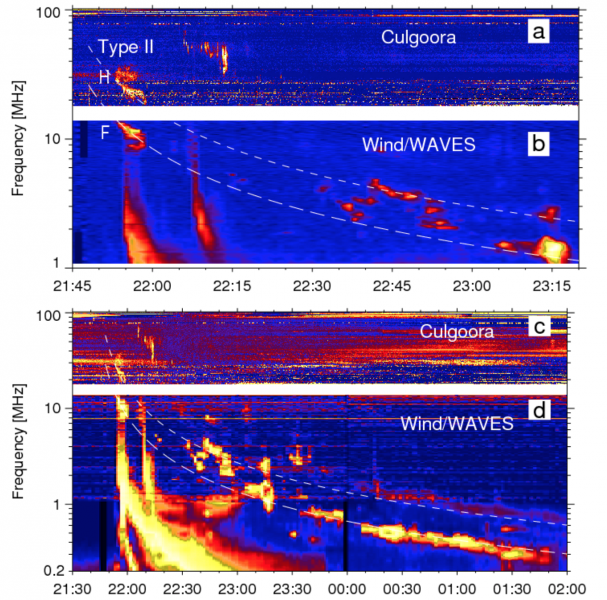
Figure 3 – Type II emission in the Culgoora and Wind/WAVES spectra and trajectories calculated for an impulsively excited piston-shock at fundamental (F, long-dashed) and harmonic (H, short-dashed) emissions.
The yellow wave fronts in Figure 4 correspond to the Type II trajectories. The wave was most likely excited by the filament top in Figure 4a near the peak of its acceleration (Figure 1), passed through the shell (future frontal structure) in Figure 4b, and appeared as a halo surrounding the CME body in Figures 4c,4d. The contrast between the decelerating shock-wave kinematics and accelerating eruptive structures disfavors the initial bow-shock excitation.
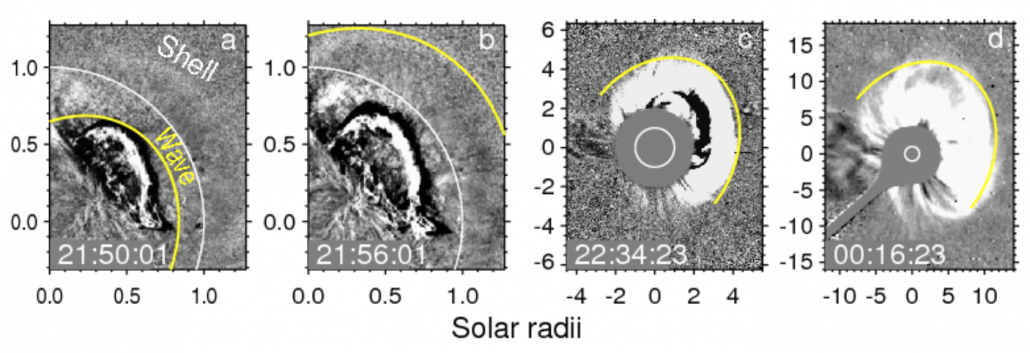
Figure 4 – Wave signatures in SDO/AIA 211 Å (a,b), SOHO/LASCO-C2 (c), and C3 (d) images along with yellow wave fronts calculated. White circles denote the solar limb.
Conclusions
The high speed of this CME event was due to considerable reconnected flux that can be underestimated in non-flare-associated events. The shock wave was most likely impulsively excited by the erupting filament in the same way as in flare-associated events and changed to the bow-shock regime later.
Based on recent paper by Grechnev V.V., Kuzmenko I.V. “A Geoeffective CME Caused by the Eruption of a Quiescent Prominence on 29 September 2013”. 2020, Solar Phys. 295, 55. DOI: 10.1007/s11207-020-01619-x
References
Cane H.V., Erickson W.C. 2005, Astrophys. J., 623, 1180
Chertok, I.M., Grechnev, V.V., Abunin, A.A. 2017, Solar Phys. 292, 62
Cliver, E.W., Kahler, S.W., Kazachenko, M., et al.: 2019, Astrophys. J., 877, 11
Gopalswamy, N., Yashiro, S., Akiyama, S., et al.: 2017, Solar Phys., 292, 65
Grechnev, V.V., Uralov, A.M., Chertok, I.M., et al.: 2011, Solar Phys., 273, 433
Pal, S., Nandy, D., Srivastava, N., et al.: 2018, Astrophys. J., 865, 4