Coronal Mass Ejections (CMEs) are hot, massive blobs of plasma and magnetic fields that erupt from the Sun, and are sometimes Earth-directed. Depending on their speed and mass these transients can strongly effect the space weather, causing geomagnetic storms and damage to space bound technologies. It is therefore imperative to understand the CME kinematics and propagation dynamics. Close to the Sun, CMEs are governed by Lorentz Forces, while they are influenced by solar wind aerodynamic drag farther out. Drag forces due to momentum coupling between the ambient solar wind and the CME can ‘drag up’ a slow CME or ‘drag down’ a fast one. In this nugget we describe results from our work on studying the effect of solar wind drag on slow and fast CMEs (Sachdeva et al. 2015). Our sample is a set of 8 CMEs between 2010-2011 observed using LASCO and STEREO missions. The CME observations are fitted to a 3D geometrical Flux rope model using the Graduated Cylindrical Shell (GCS) model (Thernisien et al. 2006). The height-time data is derived from this fitting technique. Assuming only solar wind drag force is acting on the CMEs, we consider a 1D aerodynamic drag model using a microphysical prescription for the coefficient of drag \(C_{D}\) (Subramanian et al. 2012) to estimate the heliocentric distances at which the drag force dominates the CME propagation.

Drag Force Model

Force due to momentum coupling interaction between the CME and solar wind can be written as:
\begin{equation}\label{eq:1}
F_{drag} = m_{cme} \frac{dV_{cme}}{dt} =- \frac{1}{2}     C_{\rm D}   A_{cme}   n   m_{p}\biggl( V_{cme} – V_{sw} \biggr)   \biggl|V_{cme}- V_{sw}\biggr|\;, \tag{1}
\end{equation}
where, \(m_{cme}\), \(A_{cme}\), \(V_{cme}\) are the CME mass, cross-sectional area and velocity respectively. $n$ is the solar wind density, \(m_{p}\) is the proton mass and \(V_{sw}\) is the solar wind speed. The drag coefficient \(C_{\rm D}\) was experimentally determined for subsonic, high Reynolds number flow past a solid body
\[C_{\rm D}=0.148-4.3 \times 10^4 Re^{-1} + 9.8 \times 10^{-9} Re \tag{2}\label{eq:2}\]
For each event, we solve the differential equation for drag \eqref{eq:1} using observed parameters and get a modeled solution for the height-time CME profile. Our sample includes one fast (CME2, speed =916 km/s ) CME and remaining slow to medium speed CMEs. Table 1 shows the CME serial number, observed date range, initial observed height and velocity.

 

No	Date	Initial Height \(h_{0}\)	Initial Velocity \(v_{0}\) km/s	\(\widetilde{h}_{0}\)	\(\widetilde{v}_{0}\) (km/s)	\(C_{\rm D}\) Range
1	2010 Mar 19-23	3.5	162	21.9	383	0.1-0.3
2	2010 Apr 03-05	5.5	916	5.5	916	0.6-1.4
3	2010 Apr 08-11	2.9	468	19.7	506	0.2-0.4
4	2010 Jun 16-20	5.7	193	15.2	437	0.2-0.3
5	2010 Sep 11-14	4.0	444	27.7	490	0.4-0.6
6	2010 Oct 26-31	5.3	215	20.1	445	0.25-0.5
7	2011 Feb 15-18	4.4	832	39.7	530	0.25-0.4
8	2011 Mar 25-29	4.8	47	46.5	456	0.25-0.35

Table 1- Col1-Serial number; Col2-Observed date range for CME; Col3-Initial observed height; Col4-Initial CME speed;Col5-height at which the model is later initiated; Col6-velocity at this later height;Col7-Range of drag coefficient values from Equation \eqref{eq:2}.

Fast CME-CME 2

On 2010 April 03, there was a fast CME with Sun-Earth travel time of approximately 60 hours. The initial speed derived from the height-time GCS data for this event is 916 km s\(^{-1}\). Using the first observed time point as the initial condition for the drag model, we solve the equation to get the predicted height-time profile for the CME.

We use the above mentioned drag coefficient prescription in our model and find that the observed height-time profile and the modeled solutions are in good agreement. In Figure 1, the plot for CME2 shows diamonds as the data points and the red dash-dotted line is the predicted trajectory of the CME using the drag-only model. This exercise resonates with the general knowledge that fast CMEs are slowed down by the solar wind from very early on.

CME2 plot in Figure 1 also shows the modeled results using constant values of the drag coefficient. The green and brown dash-dotted lines represent model solutions corresponding to \(C_{\rm D}\) of 0.1 and 5 respectively. The discrepancy in data and model predictions shows that a reasonable range of values for the drag-coefficient is provided by the above prescription for which the data and model agree well. We get an error of 14 % in estimating the CME arrival time at the Earth.

Slow CMEs

Some literature suggests that propagation of slow CMEs is dominated by solar wind drag from very early on or after only a few solar radii. In order to understand the dynamics of slow CMEs we apply the above method to all remaining events. Drag force equation is solved from the first observed time point and the solution is shown in Figures 1 and 2 as the red dash-dotted line. We find a huge discrepancy in the observed height-time trajectory and model solution which suggests that the solar wind drag cannot satisfactorily describe the CME dynamics when started from the first observed time point i.e. at very low heights. This remains true when we used constant values for the drag coefficient too. Therefore, in order to get the heights at which the drag is important, we initiate the model from progressively larger heliocentric distances. We solve the force equation at later heights and use the parameters corresponding to that height. In Table 1, \(\widetilde{h}_{0}\) denotes the distance at which the drag force model solutions match reasonably well with the data. At \(\widetilde{h}_{0}\) the corresponding velocity is \(\widetilde{v}_{0}\). Figures 1 and 2 show the blue solid line as the predicted height-time trajectory when the drag force-only model is initiated at \(\widetilde{h}_{0}\).

We find that solar wind drag governs the CME dynamics only above a certain height and not from very early on. In particular, for our set of CMEs this height lies between 15-50 solar radii. The solar wind accelerates or decelerates depending on how slow or fast the CME is in comparison to the solar wind speed.

It is important to note that for many events there is very little evolution beyond this height. CME 5 decelerates moderately (by 13 km/s) between 28 – 150 solar radii while CME 1 hardly decelerates.

To reiterate, the model we use is inclusive of only solar wind drag and no other force, thus, the momentum coupling between CME and ambient solar wind affects the CME propagation above these heights in case of slow CMEs. A definitive remark we stress on is that below these heights the CME is not drag dominated.

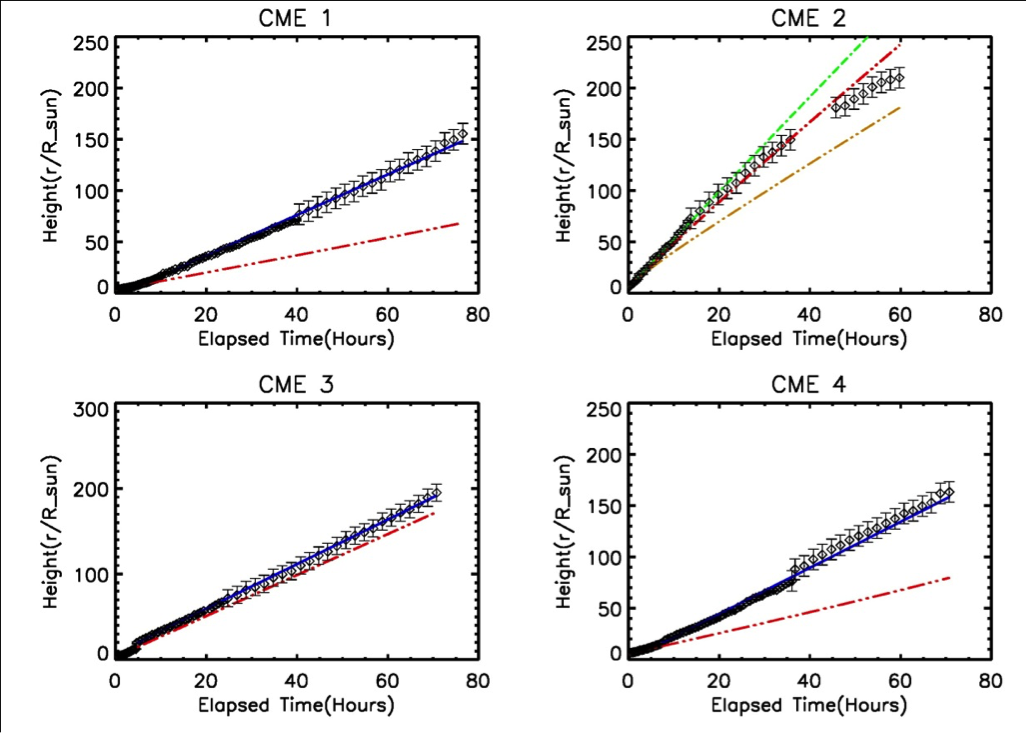
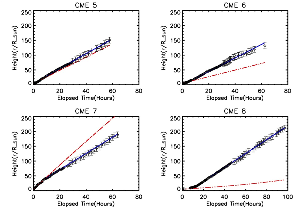
Figure 1 and 2-Diamonds- height data points along with error bars. Red dash-dotted line- model solution prediction when it is initiated from the first observed data point. Blue solid line- model predicted height-time profile when initiated at \(\widetilde{h}_{0}\).

Conclusions

We aimed at understanding the propagation dynamics of a set of CMEs by studying the action of aerodynamic drag force on these events. With a 1D model which takes into account only the interaction between CMEs and solar wind, (Lorentz forces not included), we obtain the predicted height-time trajectory. This modeled height-time solution is compared with the observed data to find the height at which the best fit is obtained. We have used two prescriptions for the drag coefficient \(C_{\rm D}\): one is from collisionless viscosity calculation (Equation \ref{eq:2}) and the other is using constant values. The predicted range for \(C_{\rm D}\) using the first prescription is given in Table 1. Constant values from within this range give us similar results for the height-time solutions, however, with starkly different \(C_{\rm D}\) values, we do not get the agreement with data (as shown with CME 2).

It is generally accepted that the Lorentz driving force for fast CMEs dies down soon after initiation, after which the decelerating drag takes over. This is what we see for the fast CME in our sample. For CME 2, the drag-based model describes the observed trajectory quite well from early on.

This is however not true for the slow CMEs. When initiated from the start, the drag model solution is very different from the observed profile. Only when initiated at later height, do we find the heliocentric distance above which the predicted and observed height-time profiles match. In particular, we find that the solar wind drag model predictions do not agree with the data below heights \(\widetilde{h}_{0}\). This height lies between 15-50 solar radii for our sample.

This work suggests that below \(\widetilde{h}_{0}\), the CME must be under the influence of other driving forces, like Lorentz Forces that may be dominating the CME propagation. Our future work is concerned primarily with these forces at lower heights.

Additional info

Author correspondence: nishtha.sachdeva@students.iiserpune.ac.in

This nugget is based on Sachdeva, N., Subramanian, P., Colaninno, R., et al., 2015 ApJ, 809, 158

References

Sachdeva, N., Subramanian, P., Colaninno, R., et al., 2015 ApJ, 809, 158

Subramanian, P., Lara, A., Borgazzi, A. 2012, GeoRL, 39, L19107

Thernisien, A. F. R., Howard, R. A. & Vourlidas, A. 2006, ApJ, 652, 763