Session 1 -- Getting image statistics

 

An obvious example is determining the statistics (and in particular the modal count) of an image. So, imagine you are logged in and the esp command has already been issued, then the following session is what would be required to examine the NDF image p2 stored in the current directory.

% histpeak

ESP HISTPEAK running.
IN - Image NDF filename /@galaxy/ > p2

At this point type in the file name, p2. The .SDF part of the name is not required. The application, in common with most ESP applications then gives you some useful information about the image in question. In particular, the image shape will give you some idea how long you will need to wait for you answers to appear.

You will find, as you use ESP applications more, that ESP applications will often volunteer a name for the IN file to be used. This name is shown at the end of the IN prompt between two `/'s. In this instance the suggested file name is galaxy. This name may be input immediately (if it is what you want) by pressing the Return/Enter key. On VAX systems, the current suggestion may be edited by pressing the tab key. You will find that many of the ESP applications will suggest answers to other prompts as well.

Filename:   p2
Title:      Raw Plate Image
Shape:      201 x 201  pixels
Bounds:     x = 1700:1900  y = 600:800
Image size: 40401 pixels
USE - Use the whole image or an ARD file /`w'/ > w

The application now prompts you for an indication of which image pixels are to be used in assessing the image pixel statistics. Frequently, you will want to use all of them, in which case your input should be `w' or `W'. This application, and all other ESP applications, are not case sensitive so both responses are treated similarly.

If you are employing ARD files (see Appendix C ) to mask out bad pixels you should input `A' or `a'. You will then be prompted for the name of the ARD file in question, in addition to those inputs shown below. It must be remembered that the name of the ARD file must be preceeded by '^ ' or the input will be interpreted as a single ARD instruction and not a file name as intended.

If, instead you opt to use all the pixels, you enter `w' in response to the USE prompt you will then be prompted as shown below with an appropriate response:

SFACT - Smoothing width you wish to use /0/ > 2
DEVICE - Display device code or name /@xw/ > ikon

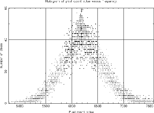
This simple set of instruction will then cause HISTPEAK to examine the NDF image p2 (a plate scan), using all its non-bad pixels. When a smoothed histogram is created by the application for determining a modal value (an unsmoothed histogram is always created as well) a Gaussian filter of radius 2 counts will be used. The histogram generated is displayed on device IKON. An example output display is shown as Figure 1 and the output to the screen is shown below.

Filename:   p2
Title:      Raw Plate Image
Shape:      201 x 201  pixels
Bounds:     x = 1700:1900  y = 600:800
Image size: 40401 pixels

HISTPEAK Results: p2

Pixels (used):              40401     Pixels (bad):                0
Lowest count:            4768.000     Highest count:        9388.000
Skewness:                   0.516     Kurtosis:                1.795

Mean:                    6226.607     Median:               6210.462

Histogram modal values:
Unsmoothed:              6179.000     Smoothed:             6214.000
Projected:               6204.297     Interpolated:         6185.874

Absolute dev.:            333.494     Variance:              183890.
Standard. dev.:           428.824     Back. st. dev.:        392.448

Smoothing filter radius:
Radius request:                 2     Radius actual:               2

Contents of the most occupied histogram bin:
Unsmoothed:                60.000     Smoothed:               52.479
Interpolated:              39.416

 

Figure 1: The unsmoothed pixel count histogram generated by HISTPEAK.

If you re-run HISTPEAK but this time input an SFACT value of 4 you will find that the results for some quantities are different. This is as you would expect when histograms are smoothed. As you can see from the excerpt below, the values affected are those relating to values extracted from the smoothed histogram. Figure 2 shows the histogram and the effect of smoothing upon the shape of the pixel count distribution - smoothed points are plotted bold.

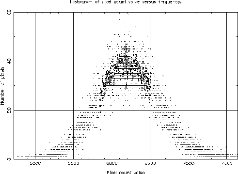
Histogram modal values:
Unsmoothed:              6179.000     Smoothed:             6176.000
Projected:               6175.306     Interpolated:         6193.840

Absolute dev.:            333.494     Variance:              183890.
Standard. dev.:           428.824     Back. st. dev.:        365.752

Smoothing filter radius:
Radius request:                 4     Radius actual:               4

Contents of the most occupied histogram bin:
Unsmoothed:                60.000     Smoothed:               46.204
Interpolated:              39.609

 

Figure 2: The smoothed pixel count histogram generated by HISTPEAK.