Quantifying the Toroidal Flux of Pre-existing Flux Ropes of CMEs
Xing, C., X. Cheng, Jiong Qiu, Qiang Hu, E. R. Priest, and M. D. Ding, Quantifying the Toroidal Flux of Pre-existing Flux Ropes of CMEs, arXiv e-prints, arXiv:1912.10623 (2019) (ADS)
(click on the image for a larger version)
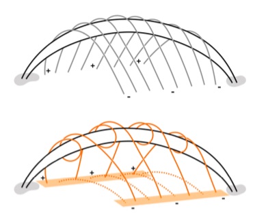
A cartoon illustrating how a "quasi-2D" view of flux ropes might suppress
vital (or at least interesting) physics.
The paper seeks quantitative estimates of the toroidal flux from field
configurations prior to eruption, certainly a worthwhile thing to do.
But here the "before" and "after" views seem to show a sudden
collapse of the distribution of current, from
a volume-filling conduction path ("before") into a concentrated flux-rope
current ("after").
This distribution is discussed in a recently-offered
Démoulin cartoon, but how can
this happen physically?
The "quasi-2D" description here implicitly avoids the discussion
of any footpoint matching to the photosphere ∇ x B condition,
but is it really OK to do this?
Note that a large number of other
cartoons seem to be assuming that the answer is "yes", but really?
A cartoon illustrating how a "quasi-2D" view of flux ropes might suppress vital (or at least interesting) physics. The paper seeks quantitative estimates of the toroidal flux from field configurations prior to eruption, certainly a worthwhile thing to do. But here the "before" and "after" views seem to show a sudden collapse of the distribution of current, from a volume-filling conduction path ("before") into a concentrated flux-rope current ("after"). This distribution is discussed in a recently-offered Démoulin cartoon, but how can this happen physically? The "quasi-2D" description here implicitly avoids the discussion of any footpoint matching to the photosphere ∇ x B condition, but is it really OK to do this? Note that a large number of other cartoons seem to be assuming that the answer is "yes", but really?