Simple Gaussian example

This page show a complete example of running nessai including setting up the logger, defining a model, configuring the sampler and finally running the sampler. The code for this example is included in example directory.

Code

#!/usr/bin/env python

# Example of using nessai

import numpy as np
from scipy.stats import norm

from nessai.flowsampler import FlowSampler
from nessai.model import Model
from nessai.utils import setup_logger

# Setup the logger - credit to the Bilby team for this neat function!
# see: https://git.ligo.org/lscsoft/bilby

output = './outdir/2d_gaussian_example/'
logger = setup_logger(output=output)

# Define the model, in this case we use a simple 2D gaussian
# The model must contain names for each of the parameters and their bounds
# as a dictionary with arrays/lists with the min and max

# The main functions in the model should be the log_prior and log_likelihood
# The log prior must be able to accept structured arrays of points
# where each field is one of the names in the model and there are two
# extra fields which are `logP` and `logL'


class GaussianModel(Model):
    """A simple two-dimensional Gaussian likelihood."""
    def __init__(self):
        # Names of parameters to sample
        self.names = ['x', 'y']
        # Prior bounds for each parameter
        self.bounds = {'x': [-10, 10], 'y': [-10, 10]}

    def log_prior(self, x):
        """
        Returns log of prior given a live point assuming uniform
        priors on each parameter.
        """
        # Check if values are in bounds
        log_p = np.log(self.in_bounds(x))
        # Iterate through each parameter (x and y)
        # since the live points are a structured array we can
        # get each value using just the name
        for n in self.names:
            log_p -= np.log(self.bounds[n][1] - self.bounds[n][0])
        return log_p

    def log_likelihood(self, x):
        """
        Returns log likelihood of given live point assuming a Gaussian
        likelihood.
        """
        log_l = np.zeros(x.size)
        # Use a Gaussian logpdf and iterate through the parameters
        for n in self.names:
            log_l += norm.logpdf(x[n])
        return log_l


# The FlowSampler object is used to managed the sampling. Keyword arguments
# are passed to the nested sampling.
fs = FlowSampler(GaussianModel(), output=output, resume=False, seed=1234)

# And go!
fs.run()

Output

In this examples the sampler with save the outputs to outdir/2d_examples/. The following is a explanation of the files in that directory.

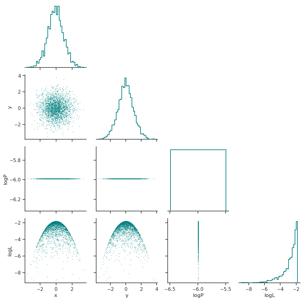
Posterior distribution

The posterior distribution is plotted in posterior_distribution.png, this includes the distributions for the parameters that were sampled and the distribution of the log-prior and log-likelihood.

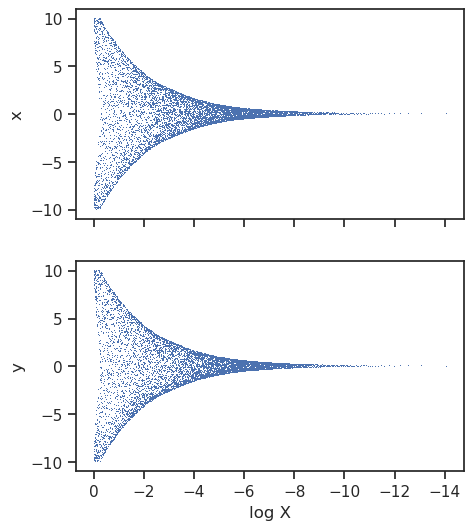
Trace

The trace plot shows the nested samples for each parameter as a function of the log-prior volume.

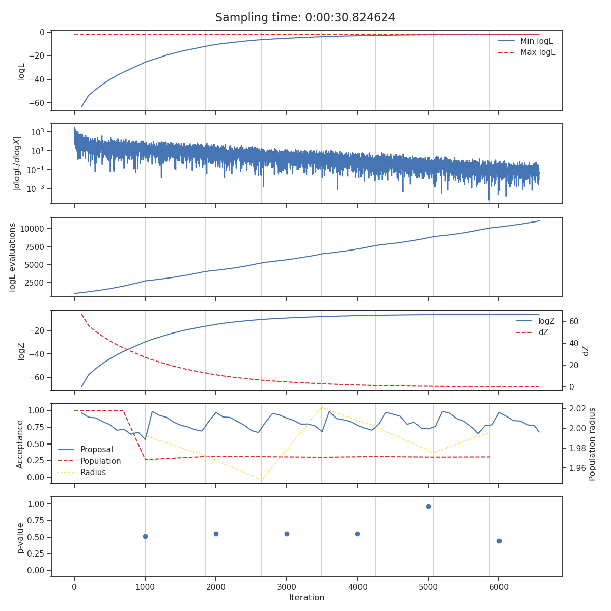
State

The state plot shows all the statistics which are tracked during sampling as a function of iteration. From top to bottom these are

The minimum and maximum log-likelihood of the current set of live points
The cumulative number of likelihood evaluations
The current log-evidence \(\log Z\) and fraction change in evidence \(\text{d}Z\)
The acceptance of the population and proposal stages alongside the radius use for each population stage.
The \(p\)-value of the insertion indices every nlive live points

The iterations at which the normalising flow has been trained are indicated with vertical lines and total sampling-time is shown at the top of the plot.

Insertion indices

The distribution of the insertion indices for all of the nested samples is shown on the left along with the expect uniform distribution and the 1-sigma bounds determined by the total number of live points. The cumulative mass function is shown on the right where the uniform function is shown with a dashed line, the overall distribution shown in blue and the distribution every nlive live point shown in light grey.

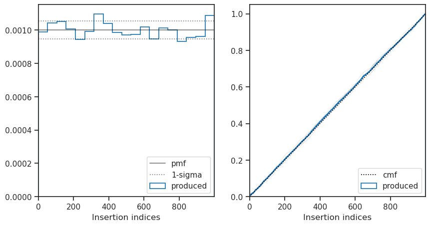
This plot is useful when checking if the sampler is correctly converged, a non-uniform distribution indicates the sampler is either under or over-constrained.