Up until now the known pulsar search has made use of code TargetedPulsars.c and HeterodynePulsar.c in LALApps, written by Rejean, and added to by me. This code has served us well, but was never meant as a final version. It requires quite a lot of knowledge of the code to run it properly and can be quite unweildy at times. To run the code a list of frame files must be created and then sorted, using a segment list, into science mode segments and then broken up into the number of jobs you want (generally dependent on how many nodes of a cluster you want to run on). Each job reads in the data from its associated file list, and then heterodynes the data using the exact phase evolution of the pulsar phase (including all Doppler delay corrections) at 16384 Hz, for each pulsar. The output is low-pass filtered and rebinned to 1/60 Hz giving our B_ks. On ce this is done the data from all the different time segments can be concatenated together to form the whole data set for each pulsar.
The main reason for changing from this process was that if things change, like the segment list, the calibration, or updated parameters are obtained, then the whole analysis must be run again. This can become time consuming. Therefore the new code must provide a way to lessen the time needed to run the analysis or at least make it more flexible to changes.
To do this it was decided to return to a heterodyne method, which was orginally used for the S1 analyses. This is a two stage heterodyne: the first part being a coarse heterodyne in which the solar system and binary Doppler delays are not included, thus speeding up the calculations, and then filtering and rebinning to 1 Hz before outputing the values; and then a second fine heterodyne which removes the Doppler delays, performs the calibration and removes outliers from the data, before outputting the final B_ks.
The coarse heterodyne stage can be run on all data in science mode, will not be calibrated and does not require the precise knowledge of the phase evolution that the full heterodyne needs. This means that it need only be performed the once and any changes to the segment lists, calibrations, or updates to the pulsar parameters can be performed in the second heterodyne at the much reduced sample rate. This second step can be performed very quickly once the coarse heterodyne has been done.
The main limitation to this method is that the coarse heterodyen stage can become rather I/O bound. This is due to the fact that the jobs on a cluster are now set up that we have 1 job per pulsar over the whole of the data stretch being studied, so all the data has to be read in for each pulsar. This is opposed to what was previously done whereby the whole data set was split up and each bit of data was only read in the once and had the heterodynes for all the pulsars perform on it. Despite this difference the codes are still comparable in speed, with the new code (in coarse heterodyne mode) analysing ~1 days data per hour for each pulsar. This should hopefully speed up when the code is made to read frames held locally on the nodes of each cluster (we see that we get ~3.15 days data per hour!).
The new heterodyne code can be found in LALApps src/pulsar/ TDS_isolated/heterodyne_pulsar.c and heterodyne_pulsar.h.
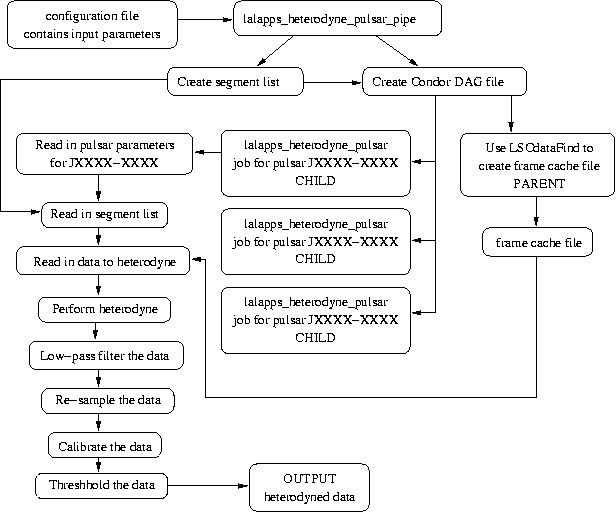
The pipeline used by the new code can be seen in the plot below.
Let us first go through the header file. The main inclusion to note are the BinaryPulsarTiming.h header file which provides the routines for reading from TEMPO .par pulsar parameter files, and the routines for calculating the binary system time delays - this is now in LAL in the pulsar package. It should also be noted that I use the frame library headers rather than the LAL frame reading headers - this is because of the ease of using the frame library routines over the LAL routines.
The USAGE macro is defined to list the command line arguments taken by the code, which will be discussed later. The other definitions all explained in their associated comment lines.
The first structure CalibrationFiles contains the paths to the associated calibration files. The FrameCache structure contains a list of all the frame file names, each ones duration and each ones start time. The InputParams structure contains general information on the type of heterodyne, filtering, segmets, parameter files needed etc. The HeterodyneParams structure contains all the necessary information to perform the heterodyne, in which all the appropriate pulsar parameters (positions, frequencies, binary elements) are contained within the BinaryPulsarParams structures.
The functions will be discussed in the next section.
This code performs the vast majority of the tasks in the analysis. What it doesn't do is obtain segment list or frame file lists, although this preprocessing is performed by a python analysis pipeline script (also within LALApps) which will be discussed later. I will describe each of the functions in turn.
int main(int argc, char *argv[]) - the main program. In this we first obtain the command lines input parameters. We then read in the pulsar parameters from it's .par file - this is done twice if we have an updated parameter file. We then set the detector location. We then get the data segment lists. For the coarse heterodyne we read in the list of frame files, their start times and durations, from the frame cache file. If a filter knee frequency is defined we set up the filters. We then set up the output file for the heterodyned data. We then enter the main loop. For the coarse heterodyne this will loop over all the data, reading in and heterodyning chunks of MAXDATALENGTH at a time. For the fine heterodyne this loop will only be implemented once. For the coarse heterodyne case, we firstly get a list of the frame files that cover the section of time we need. We then read in the data from the frames. We put the data into a COMPLEX16TimeSeries with the imaginary part set to zero. If we are performing a fine heterodyne we just reading in the complex data, including timestamps from the given input file. Once the data has been read in it is heterodyned. If the filter knee frequency is set it is filtered (this filter knee frequency defaults to zero if it is not given as a command line argument - therefore no filtering will be performed). If a coarse heterodyne has been performed then we will not have created a vector of time stamps, so this is not initialised. We then resample the data to a lower rate. If the calibration flag is set then we calibrate the data (default is to not calibrate). If the threshold flag is non-zero then we veto data above the given threshold (default is to not perorm the vetoing). We then output the data.
void get_input_args(InputParams *inputParams, int argc, char *argv[]) - this function uses get_opt to read and parse the command line arguments listed below:
void heterodyne_data(COMPLEX16TimeSeries *data,
REAL8Vector *times, HeterodyneParams hetParams) - this function takes in the time series
of data, the time stamps for each point (required because the times between data aren't uniform
over the whole data set i.e. there are gaps between data segments) and the heterodyne parameters.
The first thing it does is set the epochs of the position and frequency if one or other is not
defined - for example if the position epoch is not defined then it is set equal to the frequency
epoch and vice versa. If we are performing a fine heterodyne (heterodyneflag > 0) then we do the same for the fine heterodyne (or updated)
parameters. The next thing is to set up the solar system ephemeris files if we are performing a fine
heterodyne. We then enter the loop in which the heterodyne is performed. If we are doing a coarse
heterodyne we set the time stamp for the data point, otherwise we read the time stamp from the times vector. We then calculate the coarse phase at this
time, using all the frequency derivatives we have - this is required for both the coarse and the
fine heterodynes as the fine heterodyne calculates the difference between the two. If performing the
fine heterodyne we set the pulsar position, including updates from any proper motions. We then set
the number of leap seconds between GPS and UTC - at the monent this is 14 seconds, but for earlier
data it was 13 seconds. We then use LALBarycenter to
calculate the time delay to the solar system barycentre. If we have a binary system, we then
calculate the time delay to the binary system barycentre. These time delays are then added to the
time of the data point, and the epoch of the pulsar parameters subtracted (this being the zero of
the phase). The phase is then recalculated with the time delay corrections included. The heterodyne
uses the equations below.
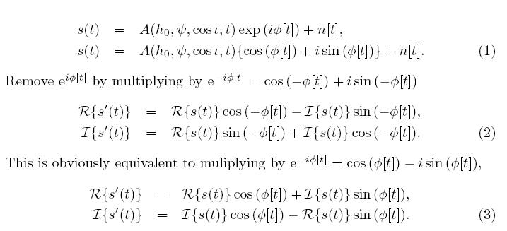
If we are performing just the coarse heterodyne then we calculate the modulus of the coarse phase, but for the fine heterodyne, we calculate the difference between the fine heterodyne phase and the coarse phase. This phase is then used to heterodyne the data (for the coarse heterodyne the imaginary part of the data has already been set to zero in the main program).
void get_frame_times(CHAR *framefile, REAL8 *gpstime, INT4 *duration) - this function takes in a frame file name and returns the GPS time and duration as extracted from the file name. This function is currently not used in the program as the frame files are read in from a frame cache file already containing the time and duration of the file.
REAL8TimeSeries *get_frame_data(CHAR *framefile, CHAR *channel, REAL8 time, REAL8 length, INT4 duration) - this function takes in a frame file name, the frame channel name, the time at which we want to read data from, the length of data we want to read in (in samples), and the duration os data (in seconds). It returns a REAL8TimeSeries containing the data. We firstly attempt to open the frame file. If this is sucessful we allocate memory for the data and set the channel name. We then use FrFileIGetV to read the data from the frame file. We then determine, from the channel name, if the data has been read in as double precision (as is the case for calibrated h(t) data from GEO600 data and LIGO) or single precision (as for uncalibrated LIGO data). We then fill in the REAL8TimeSeries.
void set_filters(Filters *iirFilters, REAL8 filterKnee, REAL8 samplerate) - this function takes in a pointer to a Filters structure, the knee frequency of the filter, and the data sample rate. This function is the same a section of the old driver code and creates three third order low-pass Butterworth filters. Firstly it sets the zeros, poles and the gain of a ZPG filter and then from this ZPG filter it creates the three IIR filters.
void filter_data(COMPLEX16TimeSeries *data, Filters *iirFilters) - this function takes in the complex heterodyned data and the Filters structure that has just been created. It applies the three third order IIR filters consecutively to the data to give an overall nineth order filter.
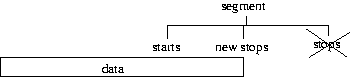
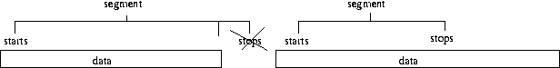
COMPLEX16TimeSeries *resample_data(COMPLEX16TimeSeries *data, REAL8Vector *times, INT4Vector *starts, INT4Vector *stops, REAL8 sampleRate, REAL8 resampleRate, INT4 hetflag) - this function takes in the complex heterodyned data, a vector of the time stamps of each data point, vectors of the start and end times of the data segments (from the segment list used), the sample rate of the data, the resample rate to be applied to the data, and the type of heterodyne performed. The function will rebin the data at the new sample rate and set the times of the data points. It will also crop any data outside of the segment list. In the definition of length we calculate the maximum number of data points in the rebinned data set. In the definition of size we calculate how many points will need to be used to rebin from the sample rate to the resample rate (this will be 16384 in the coarse heterodyne going from 16384 Hz to 1 Hz, and will be 60 for the fine heterodyne going from 1 Hz to 1/60 Hz). If we are performing a coarse heterodyne then the entire data set will have come from the same segment, so we just average the data from all the chunks of size size and put them into the new smaller output vector. We also create the time stamp of each rebinned point as the time halfway between the first and last data point. For a fine heterodyne this process is more complicated as we have to make sure that the data is within, possibly new, segment lists. We loop through all the segments, first making sure that the data is within a segment. If some of the data is within a segment and some outside a segment, then we adjust the segment accordingly. If there are gaps in the data within a segment, then we split the segment in two around the gap. We then take the average, and rebin, as before and calculate the new time stamp (again halfway between the first and last point).
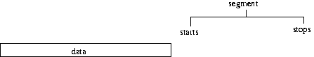
We have pointers to two vectors called starts and stops containing the start times and end
times of each segment respectively. Each entry represents one segment as read in from the segment
list file and is indexed by the variable i. We want
to loop though the lists of segment start and stop times and resample only the data within given
segments. The first if statement checks whether our data time is completely before a segment.
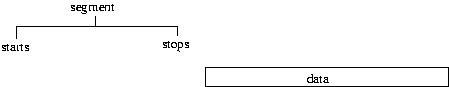
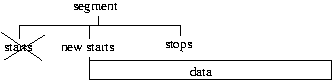
The next if statement checks whether there is an overlap between the data and the start of a
segment. If this is the case it sets a new start time for the segment as the time stamp of the
data.
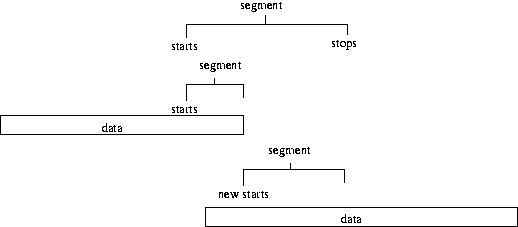
The third if statement checks if the segment overlaps the end of the data and if so sets the stop
time of the segment to the end of the data.
The final if statement checks whether the segment is after the last bit of data and if so will end
exit the resampling loop.
The next thing the code will do is use a while statement to find the first data point within the current segment looping through the j counter. As that point is the first within a segment we can set the start time of that segment to the time of the data - in reality this is just repeating what is done in the second if statement. We then set the duration of the segment by subtracting the starts time of the current segment from the end time.
We then want to check whether or not the data is actually contiguous within this segment, or whether
we have some repeated data. To do this we set up a for loop over the data which is supposed to be
within the segment i.e. duration (in seconds) times the sample rate. We first check whether there
is repeated data by testing that the data time stamps increase. If we find that the time stamp
decreases then we know we have some repeated data. We then take the data up to the point at which
the repeat occurs as our first segment and calculate the duration. We then want find the point in
the data at which we've got past the repeated data and set this as the start time of the new
segment. As we place the start time of the new segment we have to decrease the segment counter by
one, so that it repeats the same counter position in the next go of the loop. We don't have to do
anything with the stop time of the segment. In the next go of the loop the position in the data
vector, as set by the j counter, will find the right
place in the data for the next segment. So basically we just ignore any repeated data.
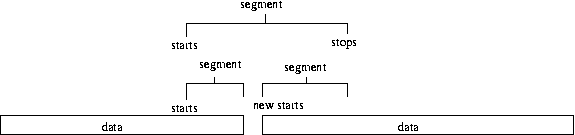
We also check whether the data is contiguous within a segment i.e. that all the
points are only separated by 1/sample rate (generally 60 seconds in our case). If there is a break
in the data wihtin a segment then that segment will be split in two. As above the duration of
the data before the break is calcated (and will be used in the subsequent resampling), and the
start time of the new segment is set as the point after the break in the data. Again we place this
new start time into the position of the previous start time, so have to decrease the i counter by
one so this new segment is used.
This process will also work if there is a break in the data before the end of a segment, but the
next point is after the end of that segment. The start of the new segment is set using the timestamp
of the first data point after the break, which in this case will be greater than the last point in
the current segment. We check for this and if it is the case then we don't decrease the segment
number i, so in the mext loop we will move onto the
next actual segment.
INT4 get_segment_list(INT4Vector *starts, INT4Vector *stops, CHAR *seglistfile) - the function takes in the name of a file containing the segment lists in segwizard format, and outputs all the start and end times. It first attempts to open the file, we then ignore any comments, and read in the start and end times. It returns the number of segments.
CHAR *set_frame_files(INT4 *starts, INT4 *stops, FrameCache cache, INT4 numFrames, INT4 *position) - this function takes in the science segment start and end times, the frame cache containing the list of all frames, their start times and durations, the number of frames, and the position within segments. The amount of data read in at one time is determined by MAXDATALENGTH. We want to create a smaller list just containing the frames covering the amount of data needed, this will be smalllist. We compare the start times of the frame files with the times of the science segments. For the first frame within a science segemt we start making smalllist, and then concantenate subsequent frames onto it until we've got all those within MAXDATALENGTH. If we don't include all of a segment within MAXDATALENGTH then we augment it's start time and move the position within the segemnts back one.
void calibrate(COMPLEX16TimeSeries *series, REAL8Vector *datatimes, CalibrationFiles calfiles, REAL8 frequency) - this function takes in the heterodyned and rebinned time series, the times of each data point, a CalibrationFiles structure containing the calibration files, and the pulsar gravitational wave frequency. If the calibration response function is the only file given then this will be used to perform the calibration, however if the sensing function, open loop gain and calibration coefficient files are given then these will be used to perform the calibration. The first part checks if the calibration coefficients are available and if not read in the response function. This is then multiplied by the complex time series of data. If the calibration coefficients are given then we need to read in the sensing function, open loop gain and coefficients from their respective files. These assume that in the calibration files any comments are given by the % sign. We then make sure that the calibration coefficients cover the span of the data that we have. We then loop over the data and the calibration coefficients, matching them in time (closest within plus or minus 30 secs), calculating the corresponding response function and calibrating the data. We veto any data that has associated calibration coefficients outside the range ALPHAMIN to ALPHAMAX - this will include points where the coefficients are zero. We then resize the data incase any data has been cut out due to the coefficient veto.
void get_calibration_values(REAL8 *magnitude, REAL8 *phase, CHAR *calibfilename, REAL8 frequency) - this function reads in a calibration file, and returns the calibration values amplitude and phase and the given frequency. The function works under the assumption that any comments with the caliration files are prefixed by a %, and that the values are an ascii text list three column wide with: frequency amplitude phase.
void remove_outliers(COMPLEX16TimeSeries *data, REAL8Vector *times, REAL8 stddevthresh) - this function takes in the times series of data and the associated time stamp vector, and a standard deviation threshold above which data will be vetoed. The standard deviation of the data is calculated (assuming a mean of zero) and then any mod(data) (real or imaginary) which cross this threshold are removed. The data time series and times veectors are then resized to their new length.
This code in essense performs the same functions as the old code, things are just rearranged in a slightly different order. In the old code the entire heterodyne was done in one go before the filtering and rebinning took place, whereas now the data can be filtered and rebinned after the first heterodyne, before applying the rest of the heterodyne. However, the results of the code should still be very similar, or else something is wrong. To test some S4 data was heterodyned (for pulsar J1910-5959B) using both the old code and the new code. A filter knee frequency of 1.5 Hz was chosen - this was larger than the 0.5 Hz used in the old analyses, but meant that when the data was coarse heterodyned and rebinned to 1 Hz it had a flat spectrum over the central frequency region. The output B_ks of both codes, after the full heterodyne, are plotted against each other below.
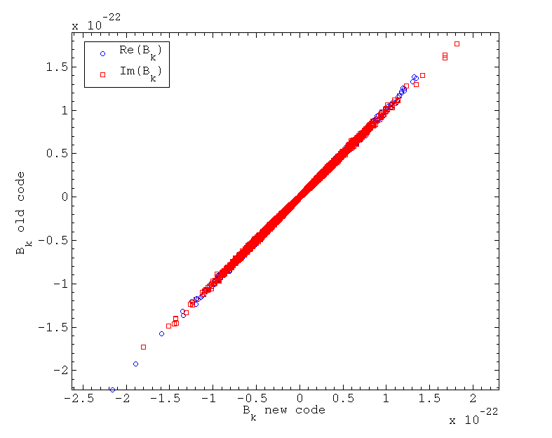
It can be seen that there is a very strong correlation between the data points produced with the new code and old code, with a standard deviation of the difference between the two set of B_ks being at the 5% level.
Another obvious check is whether the new code can extract the pulsar hardware injections. Below is a plot of the real and imaginary parts of the B_ks for the injection of PULSAR4 in S4.
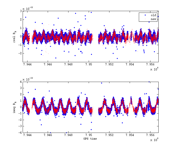
It can be seen that exactly the same signal form has been extracted by both codes.
In extracting the pulsar injection it also provided a test of whether the code works when you are
performing the fine heterodyne with updated parameters. This was because the initial
coarse heterodyne was accidentally performed with the pulsar epoch slightly wrong. The B_k
s produced when the fine heterodyne was performed with these slightly wrong values can be seen
below.

It can be seen that the signal is distorted from the true signal which was seen when the fine heterodyne was performed using the correct values of the epoch parameter.
These to checks provide strong evidence that the two codes are performing essentially the same operation.
I've tested using a couple of different filter knee frequencies to see what difference it makes on the output B_ks. These two knee frequencies are 1.5 Hz and 0.25 Hz. I've also tested the difference between resampling the data using a box car filter (i.e. averaging the samples) which provides another level of low pass filtering, against just taking one sample as our value, which doesn't provide any extra filtering. These tests have been performed for two different pulsars: the Crab pulsar, which at a frequency of 59.6 Hz is very close to the 60 Hz power line; and pulsar J0024-7204E, which at 565.6 Hz is in a relatively clean band.
The B_ks for the Crab pulsar after first the coarse heterodyne and then the fine heterodyne can be
seen in the plots below.
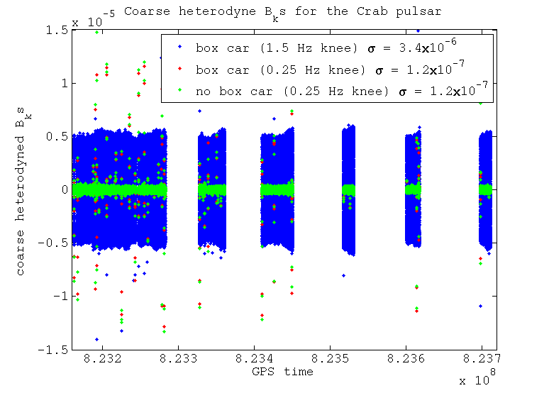
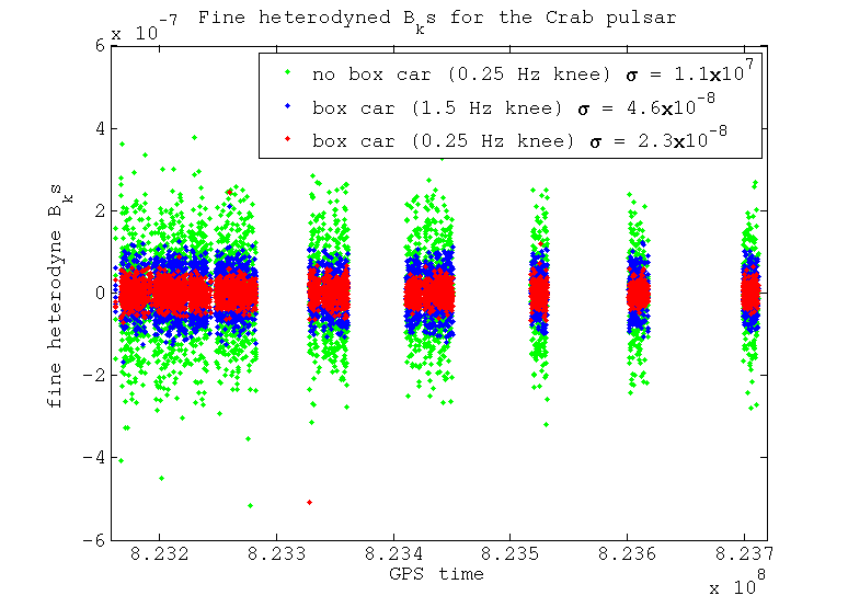
It can be seen that after the coarse heterodyne if we use the wider filter then the noise floor is a lot larger. This could be due to the filter being no where near tight enough to exclude the 60 Hz power line. With the narrower filter there will however be supression of this line. There is no major difference between using the box car averaging or not if we use the narrow filter, when resampling from 16384 Hz to 1 Hz.
When we perform the fine heterodyne and resample from 1 Hz to 1/60 Hz things start to look different. In this stage there is no more filtering using the Butterworth low-pass filter, the only filtering that would take place is that from the box car averaging when resample. We can see that if we don't apply the bow car averaging then noise that has been aliased in is not being supressed, whereas when we do average this is supressed far more. This averaging helps the data that was originally low-pass filtered at 1.5 Hz a lot, but still does not supress enough of the noise to compete with the data that was originally low-pass filtered at 0.25 Hz.
The B_ks for pulsar J0024-7204E after the coarse heterodyne and then the fine heterodyne are seen
below.
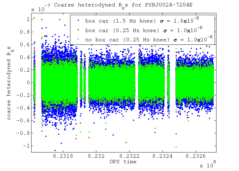
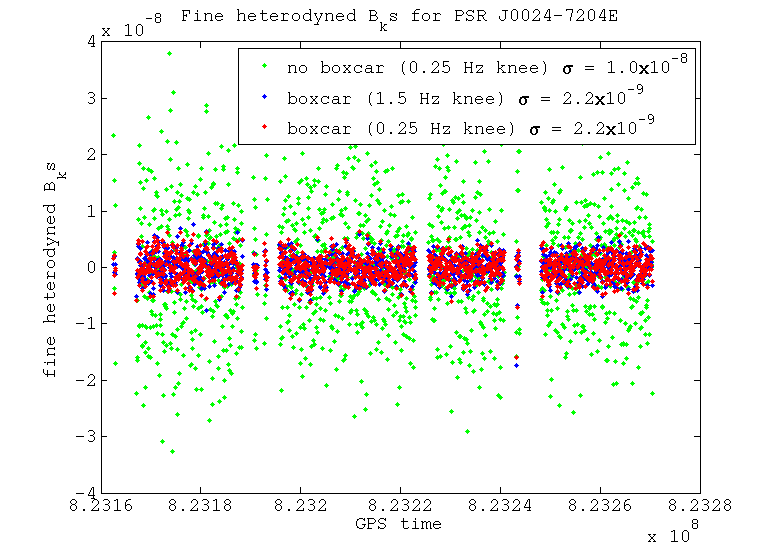
For this case where there is no large spectral disturbance near our heterodyne frequency the narrower filter makes less difference when compared with the wider filter, especially after the fine heterodyne stage. Again the box car averaged data and that without this look very similar after the coarse heterodyne. When we look at the fine heterodyne output, however, the box car averaged data is far better than that without it, due to the extra level of filtering of aliased noise that it provides.
An analysis pipeline to make the whole analysis easier to perform and reproduce has been constructed. This makes use of glue to construct a python script to find the analysis segments and build condor dags to perform the data finding and heterodyning. The pipeline scripts are available in the LALApps cvs repository as lalapps_heterodyne_pulsar_pipe and heterodyne_pulsar.py, with an example configuration file heterodyne_pulsar_coarse.ini.