Session 6 -- Looking at the image background variation

  In this session, the ESP application SKEW is employed to show what parts of a source image suffer from poor flat fielding. Before you run this program you should run HISTPEAK for the source image to determine its background value and also its associated standard deviation.

Then, the session will go something like this:

% skew
 
ESP SKEW running.

IN - Image NDF filename /@skew/ > cnt4141c
Filename:   cnt4141c
Title:      Source Image
Shape:      525 x 520 pixels
Bounds:     x= 1:525  y= 1:520
Image size: 273000 pixels
OUT - Output NDF filename /@skew/ > skew
WIDTH - Template width (in arcsec) /8/ > 
PSIZE - Pixel size /1/ > .88
MODET - Use a global mode value (y/n)? /YES/ > 
BACK - Background sky value /6200/ > 22716
USEALL - Include very bright pixels (y/n)? /NO/ > 
SIGMA - Standard deviation of the image pixels /390/ > 56
NSIGMA - Level of the cutout in SIGMA /10/ > 
MULT - Output skewness multiplying factor /1000/ >

The parameters IN and OUT refer to the source image and the output image respectively. BACK, SIGMA and PSIZE all relate to the image cnt4141c.

When the MODET option is set to FALSE, SKEW calculates a local background value when determining the skewness of each part of the image. In this example it is set to TRUE, so the image's global background value is used instead. This is the faster option.

USEALL and NSIGMA are used to define a pixel count cutoff value. If one of the image pixels is brighter than the global background (BACK) plus a certain number (NSIGMA) of background value standard deviations (SIGMA) it is excluded from the calculations. This may be used to reduce the influence of cosmic rays and other bright image features which might otherwise dominate the output.

Since skewness values are usually fairly small, a multiplying factor may be applied to all the skewness values calculated. This is specified by MULT.

Finally, SKEW shows you what it is currently doing and how far it has got. This is because, for large images, it can take a considerable time to run, especially, if the template size is large.

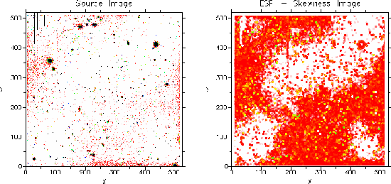
Figure 6 shows a source image and the image generated by SKEW when it was sampled over boxes approximately 10x10 pixels in size. Note how the previously unnoticed bad column (slightly left of centre near the top) is easily spotted and how large the full extent of the poor flatfielding is.

Applying SKEW to file: cnt4141c
Results file will be:  skew
Global background value used.
High count cutoff was used.
 
Percentage done so far: 10
Percentage done so far: 20
Percentage done so far: 29
..........................
..........................
Percentage done so far: 98

 

Figure 6: A poorly flatfielded source image and the output generated by SKEW.