Tutorial: Introduction to solar soft, solar radio (and auxiliary data)

Prepared by Eduard Kontar

All tutorial files can be downloaded here: http://www.astro.gla.ac.uk/users/eduard/lectures/cesra/

(last updated: 23/08/2015 21:43)

Pre-school installation guide for IDL, SSW and Perl (here)

To upgrade SSW (requires Perl installation) (extensive FAQ here)

IDL> ssw_upgrade,/loud,/spawn,/passive_ftp

To check your installation open RHESSI GUI

IDL> hessi

To add new instrument (e.g. Nancay which is a part of radio package):

IDL> setssw_windows, /nrh

* Following instruments selected:

radio/nrh

* Mission level setup files

* Instrument level setup files

* Personal startup files

Executing:    C:\ssw\site\setup\PERSONAL_STARTUP_WINDOWS.pro

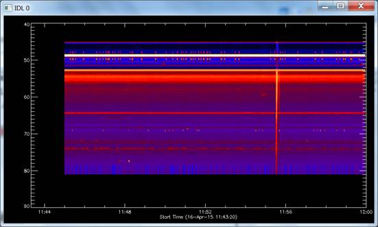
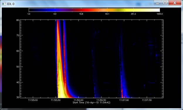
Plotting dynamic radio spectrum

To analyse and plot the radio spectrum, use IDL based solar software SSW with ‘radio’ package required (documentation is available here). As an example, one can use this simple code

IDL> radio_spectro_fits_read,'GLASGOW_20150416_114500_59.fit',data,time,freq

IDL> loadct,5

% LOADCT: Loading table STD GAMMA-II

IDL> spectro_plot,data,time,freq

% Compiled module: SPECTRO_PLOT.

% Compiled module: SPECTRO_PLOT2.

% Compiled module: AXIS_GET_EDGES.

% Compiled module: AXIS_GET_EXPANDED_RANGE.

% Compiled module: INTERP_IMAGE.

% Compiled module: INTERPOL.

% Compiled module: CSCALE.

% Compiled module: DSCALE.

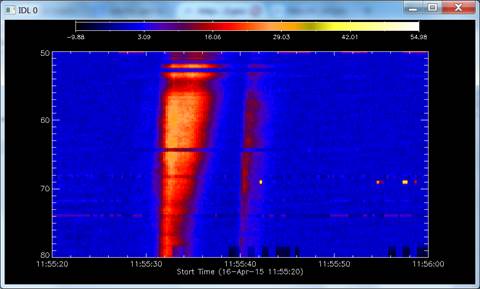
IDL> trange='2015-Apr-16 '+['11:55:20','11:56:00']

IDL> spectro_plot2,data,time,freq,timerange=trange, yrange=[50,80]

IDL> data_bg = constbacksub(data,/auto)

% Compiled module: CONSTBACKSUB.

Running Constant Backsub algorithm Version 2.1

% Compiled module: AVG.

% Compiled module: SIG_ARRAY.

% Compiled module: AVERAGE.

% Compiled module: WHERE_MISSING.

% Compiled module: IS_NOT_MISSING.

Restoring LOFAR dynamic spectrum:

IDL> restore,'total_lofar_ds.sav',/v

% RESTORE: Portable (XDR) SAVE/RESTORE file.

% RESTORE: Save file written by eduard@helios, Sun Aug 23 16:48:05 2015.

% RESTORE: IDL version 8.3 (linux, x86_64).

% RESTORE: Restored variable: DS.

IDL> help,ds

** Structure <12bcc530>, 4 tags, length=297376520, data length=297376520, refs=1:

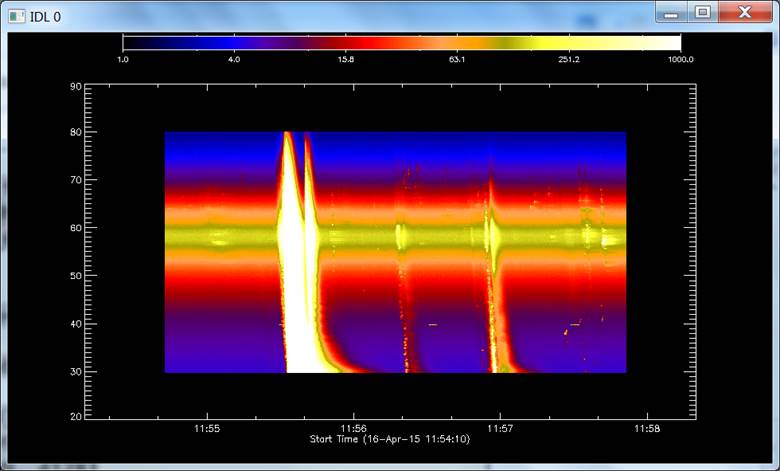
TITLE STRING 'L340180 observation total beam integrated Stokes_0'

FREQS DOUBLE Array[4128]

TIME DOUBLE Array[17999]

STOKES_0 FLOAT Array[17999, 4128]

Plotting the data:

IDL> spectro_plot2,ds.stokes_0,ds.time,ds.freqs,/log,drange=[1,1000]

IDL> normds=rebin(ds.stokes_0[0,*],17999,4128)

IDL> spectro_plot2,ds.stokes_0/normds,ds.time,ds.freqs,/log,drange=[1,1000],trange='2015-Apr-16 '+['11:55:00','11:57:00'],/xs,yrange=[30,80]

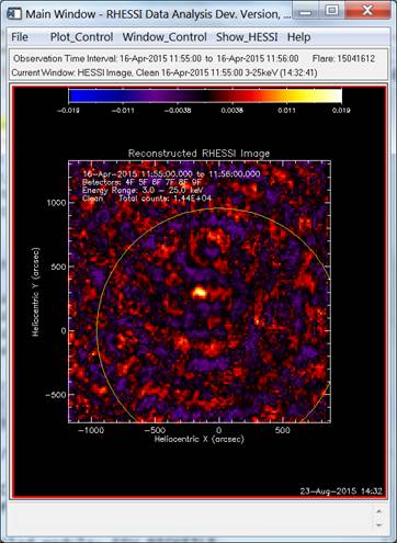
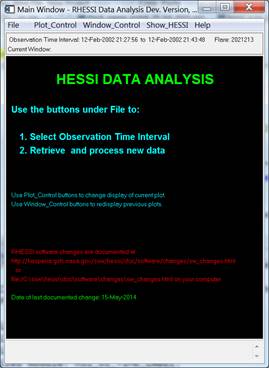
RHESSI and X-ray images

Let us make RHESSI images using GUI of RHESSI software. The details about how RHESSI imaging can be found at RHESSI pages (http://hesperia.gsfc.nasa.gov/rhessi3/pics/rhessi_imaging_kontar_2009.pdf)

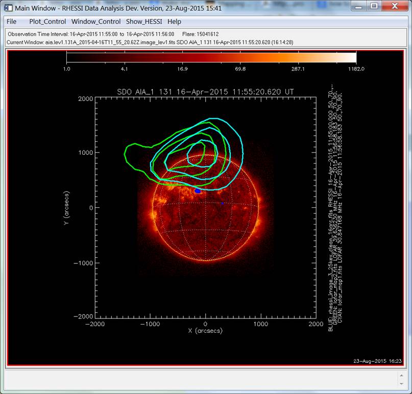
SDO and EUV images:

IDL> a = vso_search(trange[0],trange[1], wave='131', inst='aia',/url)

Records Returned : JSOC : 4/4

Records Returned : SDAC_AIA : 0/0

IDL> help,a

A STRUCT = -> VSORECORD Array[4]

Checking the data location:

IDL> print,a.url

Downloading the files:

IDL> b = vso_get(a)

% Compiled module: VSO_GET.

% VSO_GET: This will download 4 file(s)

Checking if files downloaded:

IDL> afiles=findfile('aia*.fits')

IDL> print,afiles

aia.lev1.131A_2015-04-16T11_55_20.62Z.image_lev1.fits aia.lev1.131A_2015-04-16T11_55_32.62Z.image_lev1.fits

aia.lev1.131A_2015-04-16T11_55_44.62Z.image_lev1.fits aia.lev1.131A_2015-04-16T11_55_56.62Z.image_lev1.fits

Combining images using plotman

Plotman (PLOT MANAGER (see details here http://hesperia.gsfc.nasa.gov/ssw/gen/idl/plotman/doc/plotman_help.htm)) software to manipulate various maps.

Or using RHESSI GUI and synoptic data access